# 23.2.13 DEFORMATION PLASTICITY Products: Abaqus/Standard Abaqus/CAE # References • “Material library: overview,” Section 21.1.1 • “Inelastic behavior,” Section 23.1.1 • \*DEFORMATION PLASTICITY • “Defining deformation plasticity” in “Defining other mechanical models,” Section 12.9.4 of the Abaqus/CAE User’s Guide, in the HTML version of this guide # Overview The deformation theory Ramberg-Osgood plasticity model: • is primarily intended for use in developing fully plastic solutions for fracture mechanics applications in ductile metals; and • cannot appear with any other mechanical response material models since it completely describes the mechanical response of the material. # One-dimensional model In one dimension the model is $$ E \varepsilon = \sigma + \alpha \left(\frac {| \sigma |}{\sigma^ {0}}\right) ^ {n - 1} \sigma , $$ where $\sigma$ is the stress; $\varepsilon$ is the strain; $\pmb{E}$ is Young's modulus (defined as the slope of the stress-strain curve at zero stress); $\alpha$ is the "yield" offset; $\sigma^0$ is the yield stress, in the sense that, when $\sigma = \sigma^0$ , $\varepsilon = (1 + \alpha)\sigma^0 / E$ ; and $n$ is the hardening exponent for the "plastic" (nonlinear) term: $n > 1$ . The material behavior described by this model is nonlinear at all stress levels, but for commonly used values of the hardening exponent $( n \sim 5$ or more) the nonlinearity becomes significant only at stress magnitudes approaching or exceeding $\sigma ^ { 0 }$ . The one-dimensional model is generalized to multiaxial stress states using Hooke’s law for the linear term and the Mises stress potential and associated flow law for the nonlinear term: $$ E \boldsymbol {\varepsilon} = (1 + \nu) \mathbf {S} - (1 - 2 \nu) p \mathbf {I} + \frac {3}{2} \alpha \left(\frac {q}{\sigma^ {0}}\right) ^ {n - 1} \mathbf {S}, $$ where E is the strain tensor, is the stress tensor, $p = - { \frac { 1 } { 3 } } { \boldsymbol { \sigma } } : \mathbf { I }$ is the equivalent hydrostatic stress, $q = \sqrt { \frac { 3 } { 2 } \mathbf { S } : \mathbf { S } }$ is the Mises equivalent stress, $\mathbf { S } = { \boldsymbol { \sigma } } + p \mathbf { I }$ is the stress deviator, and V is the Poisson’s ratio. The linear part of the behavior can be compressible or incompressible, depending on the value of the Poisson’s ratio, but the nonlinear part of the behavior is incompressible (because the flow is normal to the Mises stress potential). The model is described in detail in “Deformation plasticity,” Section 4.3.9 of the Abaqus Theory Guide. You specify the parameters $E , \nu , \sigma ^ { 0 }$ , n, and directly. They can be defined as a tabular function of temperature. Input File Usage: \*DEFORMATION PLASTICITY Abaqus/CAE Usage: Property module: material editor: Mechanical→Deformation Plasticity # Typical applications The deformation plasticity model is most commonly applied in static loading with small-displacement analysis, where the fully plastic solution must be developed in a part of the model. Generally, the load is ramped on until all points in the region being monitored satisfy the condition that the “plastic strain” dominates and, hence, exhibit fully plastic behavior, which is defined as $$ \frac {\alpha}{E} \big (\frac {q}{\sigma^ {0}} \big) ^ {n - 1} q > 1 0 \frac {q}{E}, $$ or $$ q > \left(\frac {1 0}{\alpha}\right) ^ {1 / (n - 1)} \sigma^ {0}. $$ You can specify the name of a particular element set to be monitored in a static analysis step for fully plastic behavior. The step will end when the solutions at all constitutive calculation points in the element set are fully plastic, when the maximum number of increments specified for the step is reached, or when the time period specified for the static step is exceeded, whichever comes first. Input File Usage: \*STATIC, FULLY PLASTIC=ElsetName Abaqus/CAE Usage: Step module: Create Step: General: Static, General: Other: Stop when region region is fully plastic. # Elements Deformation plasticity can be used with any stress/displacement element in Abaqus/Standard. Since it will generally be used for cases when the deformation is dominated by plastic flow, the use of “hybrid” (mixed formulation) or reduced-integration elements is recommended with this material model. # 23.3 Other plasticity models • “Extended Drucker-Prager models,” Section 23.3.1 • “Modified Drucker-Prager/Cap model,” Section 23.3.2 • “Mohr-Coulomb plasticity,” Section 23.3.3 • “Critical state (clay) plasticity model,” Section 23.3.4 • “Crushable foam plasticity models,” Section 23.3.5 # 23.3.1 EXTENDED DRUCKER-PRAGER MODELS Products: Abaqus/Standard Abaqus/Explicit Abaqus/CAE # References • “Material library: overview,” Section 21.1.1 • “Inelastic behavior,” Section 23.1.1 • “Rate-dependent yield,” Section 23.2.3 • “Rate-dependent plasticity: creep and swelling,” Section 23.2.4 • Chapter 24, “Progressive Damage and Failure” • \*DRUCKER PRAGER • \*DRUCKER PRAGER HARDENING • \*RATE DEPENDENT • \*DRUCKER PRAGER CREEP • \*TRIAXIAL TEST DATA • “Defining Drucker-Prager plasticity” in “Defining plasticity,” Section 12.9.2 of the Abaqus/CAE User’s Guide, in the HTML version of this guide # Overview The extended Drucker-Prager models: • are used to model frictional materials, which are typically granular-like soils and rock, and exhibit pressure-dependent yield (the material becomes stronger as the pressure increases); • are used to model materials in which the compressive yield strength is greater than the tensile yield strength, such as those commonly found in composite and polymeric materials; • allow a material to harden and/or soften isotropically; • generally allow for volume change with inelastic behavior: the flow rule, defining the inelastic straining, allows simultaneous inelastic dilation (volume increase) and inelastic shearing; • can include creep in Abaqus/Standard if the material exhibits long-term inelastic deformations; • can be defined to be sensitive to the rate of straining, as is often the case in polymeric materials; • can be used in conjunction with either the elastic material model (“Linear elastic behavior,” Section 22.2.1) or, in Abaqus/Standard if creep is not defined, the porous elastic material model (“Elastic behavior of porous materials,” Section 22.3.1); • can be used in conjunction with an equation of state model (“Equation of state,” Section 25.2.1) to describe the hydrodynamic response of the material in Abaqus/Explicit; • can be used in conjunction with the models of progressive damage and failure (“Damage and failure for ductile metals: overview,” Section 24.2.1) to specify different damage initiation criteria and damage evolution laws that allow for the progressive degradation of the material stiffness and the removal of elements from the mesh; and • are intended to simulate material response under essentially monotonic loading. 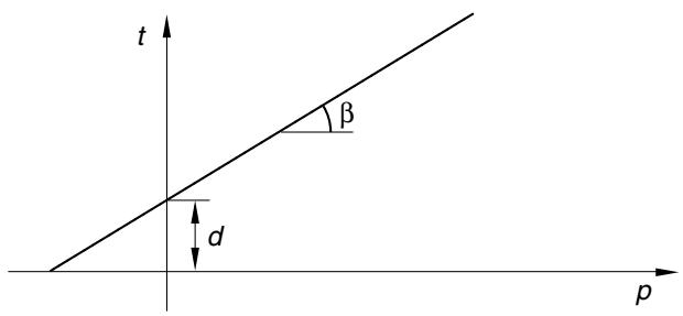# Yield criteria The yield criteria for this class of models are based on the shape of the yield surface in the meridional plane. The yield surface can have a linear form, a hyperbolic form, or a general exponent form. These surfaces are illustrated in Figure 23.3.1–1. The stress invariants and other terms in each of the three related yield criteria are defined later in this section. The linear model (Figure 23.3.1–1a) provides for a possibly noncircular yield surface in the deviatoric plane ( -plane) to match different yield values in triaxial tension and compression, associated inelastic flow in the deviatoric plane, and separate dilation and friction angles. Input data parameters define the shape of the yield and flow surfaces in the meridional and deviatoric planes as well as other characteristics of inelastic behavior such that a range of simple theories is provided—the original Drucker-Prager model is available within this model. However, this model cannot provide a close match to Mohr-Coulomb behavior, as described later in this section. 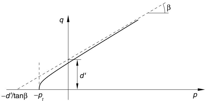The hyperbolic and general exponent models use a von Mises (circular) section in the deviatoric stress plane. In the meridional plane a hyperbolic flow potential is used for both models, which, in general, means nonassociated flow. 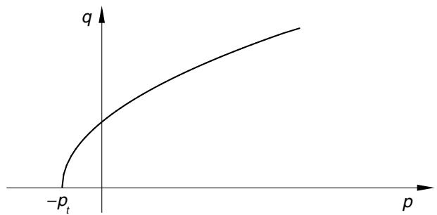The choice of model to be used depends largely on the analysis type, the kind of material, the experimental data available for calibration of the model parameters, and the range of pressure stress values that the material is likely to experience. It is common to have either triaxial test data at different levels of confining pressure or test data that are already calibrated in terms of a cohesion and a friction angle and, sometimes, a triaxial tensile strength value. If triaxial test data are available, the material parameters must be calibrated first. The accuracy with which the linear model can match these test data is limited by the fact that it assumes linear dependence of deviatoric stress on pressure stress. Although the hyperbolic model makes a similar assumption at high confining pressures, it provides a nonlinear relationship between deviatoric and pressure stress at low confining pressures, which may provide a better match of the triaxial experimental data. The hyperbolic model is useful for brittle materials for which both triaxial compression and triaxial tension data are available, which is a common situation for materials such as rocks. The most general of the three yield criteria is the exponent form. This criterion provides the most flexibility in matching triaxial test data. Abaqus determines the material parameters required for this model directly from the triaxial test data. A least-squares fit that minimizes the relative error in stress is used for this purpose. For cases where the experimental data are already calibrated in terms of a cohesion and a friction angle, the linear model can be used. If these parameters are provided for a Mohr-Coulomb model, it is necessary to convert them to Drucker-Prager parameters. The linear model is intended primarily for applications where the stresses are for the most part compressive. If tensile stresses are significant, hydrostatic tension data should be available (along with the cohesion and friction angle) and the hyperbolic model should be used. Calibration of these models is discussed later in this section. 

text_image

t β d p

a) Linear Drucker-Prager: F = t − p tan $\beta - d = 0$ 

text_image

-d'/tanβ -p_t q d' β p

b) Hyperbolic: $F = \sqrt { ( d ^ { \prime } | _ { 0 } - p _ { t } | _ { 0 } \tan \beta ) ^ { 2 } + q ^ { 2 } } - p \tan \beta - d ^ { \prime } = 0$ 

text_image

q -p_t p

c) Exponent form: $F = a q ^ { b } - p - p _ { t } = 0$ Figure 23.3.1–1 Yield surfaces in the meridional plane. For granular materials these models are often used as a failure surface, in the sense that the material can exhibit unlimited flow when the stress reaches yield. This behavior is called perfect plasticity. The models are also provided with isotropic hardening. In this case plastic flow causes the yield surface to change size uniformly with respect to all stress directions. This hardening model is useful for cases involving gross plastic straining or in which the straining at each point is essentially in the same direction in strain space throughout the analysis. Although the model is referred to as an isotropic “hardening” model, strain softening, or hardening followed by softening, can be defined. As strain rates increase, many materials show an increase in their yield strength. This effect becomes important in many polymers when the strain rates range between 0.1 and 1 per second; it can be very important for strain rates ranging between 10 and 100 per second, which are characteristic of high-energy dynamic events or manufacturing processes. The effect is generally not as important in granular materials. The evolution of the yield surface with plastic deformation is described in terms of the equivalent stress , which can be chosen as either the uniaxial compression yield stress, the uniaxial tension yield stress, or the shear (cohesion) yield stress: $$ \begin{array}{l} \bar {\sigma} = \sigma_ {c} (\bar {\varepsilon} ^ {p l}, \dot {\bar {\varepsilon}} ^ {p l}, \theta , f _ {i}) \quad \text {if hardening is defined by the uniaxial compression yield stress}, \sigma_ {c}; \\ = \sigma_ {t} (\bar {\varepsilon} ^ {p l}, \dot {\bar {\varepsilon}} ^ {p l}, \theta , f _ {i}) \quad \mathrm{ifhardeningisdefinedbytheuniaxialtensionyieldstress,} \sigma_ {t}; \mathrm{or} \\ = d (\bar {\varepsilon} ^ {p l}, \dot {\bar {\varepsilon}} ^ {p l}, \theta , f _ {i}) \quad \text {if hardening is defined by the cohesion,} d, \\ \end{array} $$ where $$ \dot {\bar {\varepsilon}} ^ {p l} $$ is the equivalent plastic strain rate, defined for the linear Drucker-Prager model as $$ \begin{array}{l} \begin{array}{l} \dot {\varepsilon} ^ {p l} \\ = | \dot {\varepsilon} _ {1 1} ^ {p l} | \text { if hardening is defined in uniaxial compression; } \end{array} \\ = \dot {\varepsilon} _ {1 1} ^ {p l} \text { if hardening is defined in uniaxial tension; } \\ = \dot {\gamma} ^ {p l} / \sqrt {3} \text { if hardening is defined in pure shear, } \\ \end{array} $$ and defined for the hyperbolic and exponential Drucker-Prager models as $$ \dot {\bar {\varepsilon}} ^ {p l} = \frac {\pmb {\sigma} : \dot {\pmb {\varepsilon}} ^ {p l}}{\bar {\sigma}}; $$ $$ \bar {\varepsilon} ^ {p l} = \int_ {0} ^ {t} \dot {\bar {\varepsilon}} ^ {p l} d t $$ $$ \theta $$ $$ f _ {i}, i = 1, 2, \dots $$ is the equivalent plastic strain; is temperature; and are other predefined field variables.