# 26.5.2 PIEZOELECTRIC BEHAVIOR Products: Abaqus/Standard Abaqus/CAE # References • “Piezoelectric analysis,” Section 6.7.2 • “Material library: overview,” Section 21.1.1 • \*DIELECTRIC • \*PIEZOELECTRIC • “Defining dielectric material properties,” Section 12.11.2 of the Abaqus/CAE User’s Guide, in the HTML version of this guide • “Defining piezoelectric properties,” Section 12.11.3 of the Abaqus/CAE User’s Guide, in the HTML version of this guide # Overview A piezoelectric material: • is one in which an electrical field causes the material to strain, while stress causes an electric potential gradient; • provides linear relations between mechanical and electrical fields; and • is used in piezoelectric elements, which have both displacement and electrical potential as nodal variables. # Defining a piezoelectric material A piezoelectric material responds to an electric potential gradient by straining, while stress causes an electric potential gradient in the material. This coupling between electric potential gradient and strain is the material’s piezoelectric property. The material will also have a dielectric property so that an electrical charge exists when the material has a potential gradient. Piezoelectric material behavior is discussed in “Piezoelectric analysis,” Section 2.10.1 of the Abaqus Theory Guide. The mechanical properties of the material must be modeled by linear elasticity (“Linear elastic behavior,” Section 22.2.1). The mechanical behavior can be defined by $$ \sigma_ {i j} = D _ {i j k l} ^ {E} \varepsilon_ {k l} - e _ {m i j} ^ {\varphi} E _ {m}, $$ in terms of the piezoelectric stress coefficient matrix, , $e _ { m i j } ^ { \varphi }$ or by $$ \sigma_ {i j} = D _ {i j k l} ^ {E} (\varepsilon_ {k l} - d _ {m k l} ^ {\varphi} E _ {m}), $$ in terms of the piezoelectric strain coefficient matrix, $d _ { m k l } ^ { \varphi }$ . The electrical behavior is defined by $$ q _ {i} = e _ {i j k} ^ {\varphi} \varepsilon_ {j k} + D _ {i j} ^ {\varphi (\varepsilon)} E _ {j}, $$ where $\sigma_{ij}$ is the mechanical stress tensor; $\varepsilon_{ij}$ is the strain tensor; $q_i$ is the electric “displacement” vector; $D_{ijkl}^{E}$ is the material’s elastic stiffness matrix defined at zero electrical potential gradient (short circuit condition); $e_{mij}^{\varphi}$ is the material’s piezoelectric stress coefficient matrix, defining the stress $\sigma_{ij}$ caused by the electrical potential gradient $E_m$ in a fully constrained material (it can also be interpreted as the electrical displacement $q_m$ caused by the applied strain $\varepsilon_{ij}$ at a zero electrical potential gradient); $d_{mkl}^{\varphi}$ is the material’s piezoelectric strain coefficient matrix, defining the strain $\varepsilon_{kl}$ caused by the electrical potential gradient $E_m$ in an unconstrained material (an alternative interpretation is given later in this section); $\varphi$ is the electrical potential; $D_{ij}^{\varphi(\varepsilon)}$ is the material’s dielectric property, defining the relation between the electric displacement $q_i$ and the electric potential gradient $E_j$ for a fully constrained material; and $E_i$ is the electrical potential gradient vector, $-\partial \varphi/\partial x_i$ . The material’s electrical and electro-mechanical coupling behaviors are, thus, defined by its dielectric property, $D _ { i j } ^ { \varphi ( \varepsilon ) }$ , and its piezoelectric stress coefficient matrix, $e _ { m i j } ^ { \varphi }$ , or its piezoelectric strain coefficient matrix, $d _ { m k l } ^ { \varphi ^ { \mathrm { ~ \tiny ~ { ~ \upsilon ~ } ~ } } }$ . These properties are defined as part of the material definition (“Material data definition,” Section 21.1.2). # Alternative forms of the constitutive equations Alternative forms of the piezoelectric constitutive equations are presented in this section. These forms of the equations involve material properties that cannot be used directly as input for Abaqus/Standard. However, they are related to the Abaqus/Standard input through simple relations that are presented in “Piezoelectric analysis,” Section 2.10.1 of the Abaqus Theory Guide. The intent of this section is to draw connections between the Abaqus/Standard terminology and input to that used commonly in the piezoelectricity community. The mechanical behavior can also be defined by $$ \sigma_ {i j} = D _ {i j k l} ^ {q} (\varepsilon_ {k l} - g _ {m k l} ^ {\varphi} q _ {m}) $$ in terms of the piezoelectric coefficient matrix $g _ { m i j } ^ { \varphi }$ , and the stiffness matrix $D _ { i j k l } ^ { q }$ , which defines the mechanical properties at zero electrical displacement (open circuit condition). Likewise, the electrical behavior can also be defined by $$ q _ {i} = d _ {i j k} ^ {\varphi} \sigma_ {j k} + D _ {i j} ^ {\varphi (\sigma)} E _ {j} $$ in terms of the dielectric matrix $D _ { i j } ^ { \varphi ( \sigma ) }$ for an unconstrained material or by $$ q _ {i} = D _ {i m} ^ {\varphi (\sigma)} g _ {m j k} ^ {\varphi} \sigma_ {j k} + D _ {i j} ^ {\varphi (\sigma)} E _ {j}, $$ where

$D_{ijkl}^{q}$	is the material’s elastic stiffness matrix defined at zero electrical displacement;
$d_{ijk}^{\varphi}$	is the material’s piezoelectric strain coefficient matrix used earlier, and based on the equations, may alternatively be interpreted as the electrical displacement $q_{i}$ caused by the stress $\sigma_{jk}$ at zero electrical potential gradient;
$g_{mkl}^{\varphi}$	is the material’s piezoelectric coefficient matrix, which can be interpreted as defining either the strain $\varepsilon_{kl}$ caused by the electrical displacement $q_{m}$ in an unconstrained material or the electrical potential gradient $E_{m}$ caused by the stress $\sigma_{kl}$ at zero electrical displacement; and
$D_{ij}^{\varphi(\sigma)}$	is the material’s dielectric property, defining the relation between the electric displacement $q_{i}$ and the electric potential gradient $E_{j}$ for an unconstrained material.

These are useful relationships that are often seen in the piezoelectric literature. In “Piezoelectric analysis,” Section 2.10.1 of the Abaqus Theory Guide, the properties $g _ { m k l } ^ { \varphi } , \ D _ { i j } ^ { \varphi ( \sigma ) }$ , and $D _ { i j k l } ^ { q }$ are expressed in terms of the properties $d _ { m k l } ^ { \varphi } , D _ { i j } ^ { \varphi ( \varepsilon ) }$ , and $D _ { i j k l } ^ { E }$ , that are used as input for Abaqus/Standard. # Specifying dielectric material properties The dielectric matrix can be isotropic, orthotropic, or fully anisotropic. For non-isotropic dielectric materials a local orientation for the material directions must be specified (“Orientations,” Section 2.2.5). The entries of the dielectric matrix (what are referred to as “dielectric constants” in Abaqus) refer to what is more commonly known in the literature as the permittivity of the material. # Isotropic dielectric properties The dielectric matrix $D _ { i j } ^ { \varphi ( \varepsilon ) }$ can be fully isotropic, so that $$ D _ {i j} ^ {\varphi (\varepsilon)} = D ^ {\varphi (\varepsilon)} \delta_ {i j}. $$ You specify the single value $D \varphi ( \varepsilon )$ for the dielectric constant. $D \varphi ( \varepsilon )$ must be determined for a constrained material. Isotropic behavior is the default. Input File Usage: \*DIELECTRIC, TYPE=ISO Abaqus/CAE Usage: Property module: material editor: Electrical/Magnetic→Dielectric (Electrical Permittivity): Type: Isotropic # Orthotropic dielectric properties For orthotropic behavior you must specify three values in the dielectric matrix $( D _ { 1 1 } ^ { \varphi ( \varepsilon ) } , D _ { 2 2 } ^ { \varphi ( \varepsilon ) }$ , and $D _ { 3 3 } ^ { \varphi ( \varepsilon ) } )$ Input File Usage: \*DIELECTRIC, TYPE=ORTHO Abaqus/CAE Usage: Property module: material editor: Electrical/Magnetic→Dielectric (Electrical Permittivity): Type: Orthotropic # Anisotropic dielectric properties otropi, and vior you must specify six values in the dielectric matrix). $( D _ { 1 1 } ^ { \varphi ( \varepsilon ) } , D _ { 1 2 } ^ { \varphi ( \varepsilon ) } , D _ { 2 2 } ^ { \varphi ( \varepsilon ) }$ , , ,D（）， $D _ { 1 3 } ^ { \varphi ( \varepsilon ) } , \bar { D } _ { 2 3 } ^ { \varphi ( \varepsilon ) }$ $D _ { 3 3 } ^ { \varphi ( \varepsilon ) } )$ Input File Usage: \*DIELECTRIC, TYPE=ANISO Abaqus/CAE Usage: Property module: material editor: Electrical/Magnetic→Dielectric (Electrical Permittivity): Type: Anisotropic # Specifying piezoelectric material properties The piezoelectric material properties can be defined by giving the stress coefficients, $e _ { m i j } ^ { \varphi }$ (this is the default), or by giving the strain coefficients, $d _ { m k l } ^ { \varphi }$ . In either case, 18 components must be given in the following order (substitute d for e for strain coefficients): $$ \begin{array}{c c c c c c} e _ {1 1 1} ^ {\varphi}, & e _ {1 2 2} ^ {\varphi}, & e _ {1 3 3} ^ {\varphi}, & e _ {1 1 2} ^ {\varphi}, & e _ {1 1 3} ^ {\varphi}, & e _ {1 2 3} ^ {\varphi}, \\ e _ {2 1 1} ^ {\varphi}, & e _ {2 2 2} ^ {\varphi}, & e _ {2 3 3} ^ {\varphi}, & e _ {2 1 2} ^ {\varphi}, & e _ {2 1 3} ^ {\varphi}, & e _ {2 2 3} ^ {\varphi}, \\ e _ {3 1 1} ^ {\varphi}, & e _ {3 2 2} ^ {\varphi}, & e _ {3 3 3} ^ {\varphi}, & e _ {3 1 2} ^ {\varphi}, & e _ {3 1 3} ^ {\varphi}, & e _ {3 2 3} ^ {\varphi}. \end{array} $$ The first index on these coefficients refers to the component of electric displacement (sometimes called the electric flux), while the last pair of indices refers to the component of mechanical stress or strain. Thus, the piezoelectric components causing electrical displacement in the 1-direction are all given first, then those causing electrical displacement in the 2-direction, and then those causing electrical displacement in the 3-direction. (Some references list these coupling terms in a different order.) Input File Usage: Use the following option to give the stress coefficients: \*PIEZOELECTRIC, TYPE=S Use the following option to give the strain coefficients: \*PIEZOELECTRIC, TYPE=E Abaqus/CAE Usage: Property module: material editor: Electrical/Magnetic→Piezoelectric: Type: Stress or Strain # Converting double index notation to triple index notation Industry-supplied piezoelectric data often use a double index notation. A double index notation can be converted easily to the required triple index notation in Abaqus/Standard by noting the convention followed in Abaqus for the correspondence between (second-order) tensor and vector notations: the 11, 22, 33, 12, 13, and 23 components of the tensor correspond to the 1, 2, 3, 4, 5, and 6 components, respectively, of the corresponding vector. # Energy balance considerations Abaqus does not account for piezoelectric effects in the total energy balance equation, which can lead to an apparent imbalance of the total energy of the model in some situations. For example, if a piezoelectric truss is fixed at one end point and subjected to a potential difference between its two end points, it deforms due to the piezoelectric effect. Subsequently if the truss is held fixed in this deformed configuration and the potential difference removed, strain energy will be generated due to the constraints. This results in an equivalent increase in the total energy of the model. # Elements Piezoelectric coupling is active only in piezoelectric elements (those with displacement degrees of freedom and electrical potential degree of freedom 9). See “Choosing the appropriate element for an analysis type,” Section 27.1.3. # 26.5.3 MAGNETIC PERMEABILITY Products: Abaqus/Standard Abaqus/CAE # References • “Material library: overview,” Section 21.1.1 • \*MAGNETIC PERMEABILITY • \*NONLINEAR BH • \*PERMANENT MAGNETIZATION • “Defining magnetic permeability,” Section 12.11.4 of the Abaqus/CAE User’s Guide, in the HTML version of this guide # Overview A material’s magnetic permeability: • must be defined for “Eddy current analysis,” Section 6.7.5, and “Magnetostatic analysis,” Section 6.7.6; • can be specified directly for linear magnetic behavior or through one or more B–H curves for nonlinear magnetic behavior; • can be isotropic, orthotropic, or (in the case of linear behavior) fully anisotropic; • can be specified as a function of temperature and/or field variables; • can be specified as a function of frequency in a time-harmonic eddy current procedure; and • can be combined with permanent magnetization. # Linear magnetic behavior Linear magnetic behavior is defined by direct specification of magnetic permeability. # Directional dependence of magnetic permeability Isotropic, orthotropic, or fully anisotropic magnetic permeability can be defined. For non-isotropic magnetic permeability a local orientation for the material directions must be specified (“Orientations,” Section 2.2.5). Isotropic magnetic permeability For isotropic magnetic permeability only one value of magnetic permeability is needed at each temperature and field variable value. Isotropic magnetic permeability is the default. Input File Usage: \*MAGNETIC PERMEABILITY, TYPE=ISOTROPIC Abaqus/CAE Usage: Property module: material editor: Electrical/Magnetic→Magnetic Permeability: Type: Isotropic # Orthotropic magnetic permeability For orthotropic magnetic permeability three values of magnetic permeability $( \mu _ { 1 1 } , \mu _ { 2 2 } , \mu _ { 3 3 } )$ are needed at each temperature and field variable value. Input File Usage: \*MAGNETIC PERMEABILITY, TYPE=ORTHOTROPIC Abaqus/CAE Usage: Property module: material editor: Electrical/Magnetic→Magnetic Permeability: Type: Orthotropic # Anisotropic magnetic permeability For fully anisotropic magnetic permeability six values $( \mu _ { 1 1 } , \mu _ { 1 2 } , \mu _ { 2 2 } , \mu _ { 1 3 } , \mu _ { 2 3 } , \mu _ { 3 3 } )$ are needed at each temperature and field variable value. Input File Usage: \*MAGNETIC PERMEABILITY, TYPE=ANISOTROPIC Abaqus/CAE Usage: Property module: material editor: Electrical/Magnetic→Magnetic Permeability: Type: Anisotropic # Frequency-dependent magnetic permeability Magnetic permeability can be defined as a function of frequency in a time-harmonic eddy current analysis. 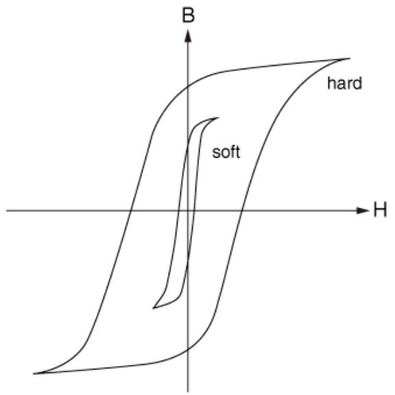Input File Usage: \*MAGNETIC PERMEABILITY, FREQUENCY Abaqus/CAE Usage: Property module: material editor: Electrical/Magnetic→Magnetic Permeability: Toggle on Use frequency-dependent data # Nonlinear magnetic behavior Nonlinear magnetic behavior is characterized by magnetic permeability that depends on the strength of the magnetic field. The nonlinear magnetic material model in Abaqus is suitable for ideally soft magnetic materials without any hysteresis effects (see Figure 26.5.3–1) characterized by a monotonically increasing response in B–H space, where B and H refer to the strengths of the magnetic flux density vector and the magnetic field vector, respectively. Nonlinear magnetic behavior is defined through direct specification of one or more B–H curves that provide B as a function of H and, optionally, temperature and/or predefined field variables, in one or more directions. Nonlinear magnetic behavior can be isotropic, orthotropic, or transversely isotropic (which is a special case of the more general orthotropic behavior). More than one B–H curve is needed to define the nonlinear magnetic behavior if it is not isotropic. # Directional dependence of nonlinear magnetic behavior Isotropic, orthotropic, or transversely isotropic nonlinear magnetic behavior can be defined. For nonisotropic nonlinear magnetic behavior a local orientation for the material directions must be specified (“Orientations,” Section 2.2.5). Isotropic nonlinear magnetic behavior For isotropic nonlinear magnetic response only one B–H curve is needed at each temperature and field variable value. Isotropic magnetic permeability is the default. Abaqus assumes that the nonlinear magnetic behavior is governed by $$ \mathbf {B} = B \left(| \mathbf {H} |\right) \left(\frac {\mathbf {H}}{| \mathbf {H} |}\right) $$ Input File Usage: You define through a B–H curve: \*MAGNETIC PERMEABILITY, NONLINEAR, TYPE=ISOTROPIC \*NONLINEAR BH, DIR=direction The B–H curve in any direction (i.e., the nonlinear behavior in global direction 1, 2, or 3) will suffice as the nonlinear magnetic behavior is assumed to be the same in all directions. Abaqus/CAE Usage: Property module: material editor: Electrical/Magnetic→Magnetic Permeability: Toggle on Specify using nonlinear B-H curve: Type: Isotropic Orthotropic nonlinear magnetic behavior For orthotropic nonlinear magnetic response three B–H curves (one curve to define the behavior in each of the local directions 1, 2, and 3) are needed at each temperature and field variable value. Abaqus assumes that the nonlinear magnetic behavior in the local material directions is governed by $$ \mathbf {B} = d i a g \left(B _ {1} \left(\left| \mathbf {H} \right|\right), B _ {2} \left(\left| \mathbf {H} \right|, B _ {3} \left(\left| \mathbf {H} \right|\right)\right) \left(\frac {\mathbf {H}}{\left| \mathbf {H} \right|}\right), \right. $$ where refers to a diagonal matrix. Transversely isotropic nonlinear magnetic behavior is a special case of orthotropic behavior, in which the behavior in any two directions is the same and is different from that in the third direction. Input File Usage: You define $B _ { 1 } \left( | \mathbf { H } | \right) , B _ { 2 } \left( | \mathbf { H } | \right)$ , and $B _ { 3 } \left( \left| \mathbf { H } \right| \right)$ , respectively, through three independent B–H curves, one in each of the directions 1, 2, and 3: ```txt *MAGNETIC PERMEABILITY, NONLINEAR, TYPE=ORTHOTROPIC *NONLINEAR BH, DIR=1 ... *NONLINEAR BH, DIR=2 ... *NONLINEAR BH, DIR=3 ... ``` Abaqus/CAE Usage: Property module: material editor: Electrical/Magnetic→Magnetic Permeability: Toggle on Specify using nonlinear B-H curve: Type: Orthotropic # Permanent magnetization Ferromagnetic materials can be magnetized by placing them in a magnetic field, which is typically created by applying currents in a system of coil windings surrounding the material being magnetized. These materials can be classified into soft and hard magnetic materials (see Figure 26.5.3–1). Soft magnetic materials lose their magnetization after removal of the applied currents (see “Nonlinear magnetic behavior”). Hard magnetic materials retain their magnetization permanently after removal of the applied currents. The leftover magnetization in a permanent magnet is called remanence, denoted by $B _ { r }$ in Figure 26.5.3–2. This magnetization can be removed by applying currents in the opposite direction; the strength of the opposing magnetic fields that remove magnetization entirely is called coercivity, denoted by $H _ { c }$ in Figure 26.5.3–2. 

text_image

B hard soft H

Figure 26.5.3–1 Response of hard and soft magnetic materials. Permanent magnetization in Abaqus is suitable for hard magnetic materials when the magnets are operating around the point of remanence. This behavior captures the response of magnetization or demagnetization around the point of remanence, as shown by the darker descending line of the hysteresis loop in Figure 26.5.3–2. The underlying magnetic permeability can be linear or nonlinear. In either case, permanent magnetization is defined by its coercivity such that $$ \mathbf {H} = \boldsymbol {\mu} ^ {- 1} \mathbf {B} - \mathbf {H} _ {c} $$ for linear isotropic, orthotropic, or anisotropic magnetic behavior and