local tangent plane with respect to the master surface facet remains fixed. Because the small-sliding formulation considers nonlinear geometric effects, Abaqus/Explicit continuously updates the orientation of the local tangent plane to account for the rotation of the master surface facet. The position of the anchor point relative to the surrounding nodes on the master surface facet does not change as the master surface deforms. # Load transfer In a small-sliding analysis the slave node will transfer load to the nodes of the master surface facet containing the anchor point, with the magnitude of the load transferred to each node weighted by its proximity to the anchor point. For example, in Figure 38.2.2–3 node 103 transmits load to both nodes 2 and 3 on the master surface. Thus, if node 103 impacts the local tangent plane, a larger share of the force would be transmitted to node 3 because it is closer to the anchor point $\mathbf { X _ { 0 } }$ . As a slave node slides along its local tangent plane, Abaqus/Explicit does not update the distribution of load transferred by a given slave node to its associated master surface nodes; the distribution is based solely on the position of the anchor point. This is unlike the small-sliding formulation in Abaqus/Standard, which does update the load distribution to the master surface nodes as sliding occurs, so that no net moment is associated with the contact forces acting on slave and master nodes per active contact constraint, regardless of the amount of sliding. Some net moment will be associated with the contact forces after sliding has occurred with the small-sliding formulation in Abaqus/Explicit. This net moment will not be significant if the sliding is truly small compared to element dimensions, but otherwise it can result in non-physical behavior and poor accounting of energy. 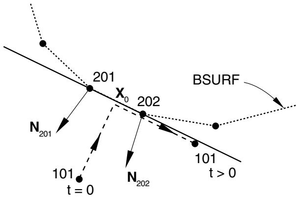Figure 38.2.2–7 shows the potential problem that arises if small sliding is used but the relative tangential motion of the surfaces is not “small.” It shows the possible evolution of contact between slave node 101 in Figure 38.2.2–1 and its master surface BSURF. Using the unit normal vectors $\mathbf { N } _ { 2 0 1 }$ and $\mathbf { N } _ { 2 0 2 }$ , the anchor point $\mathbf { X } _ { 0 }$ was found for slave node 101; for the purposes of this example, assume that it lies at the midpoint of the 201–202 face. With this location of $\mathbf { X } _ { 0 }$ the local tangent plane for node 101 is parallel with the 201–202 face. The load transfer always occurs at the original anchor point between nodes 201 and 202, no matter how far node 101 has slid along the local tangent plane. Therefore, if node 101 moves as shown in Figure 38.2.2–7, it will continue to transmit load equally to nodes 201 and 202 when, in fact, it really slid off the mesh forming the master surface BSURF. # What can be considered small sliding A contact pair in a small-sliding contact simulation should not grossly violate any of the assumptions or limitations outlined above. Adhere to the following guidelines: • Slave nodes should slide less than an element length from their corresponding anchor point and still be contacting their local tangent plane. If the master surface is highly curved, the slave nodes should slide only a fraction of an element length. • The local tangent planes formed by Abaqus/Explicit should be a good approximation of the mesh geometry; if necessary, use an initial clearance definition (“Specifying initial clearance values precisely” in “Adjusting initial surface positions and specifying initial clearances for contact pairs in Abaqus/Explicit,” Section 36.5.4) to improve the tangent plane orientation. 

text_image

201 X₀ 202 BSURF N₂₀₁ 101 t = 0 N₂₀₂ 101 t > 0

Figure 38.2.2–7 Excessive sliding in a small-sliding contact analysis. • The rotation and deformation of the master surface should not cause the local tangent planes to become a poor representation of the master surface during the course of the analysis. # Master surface refinement in small-sliding problems The basic guidelines for pure master-slave contact given previously in this section should still be followed in a small-sliding simulation. However, in a small-sliding simulation more thought must be given to the degree of refinement for the master surface. 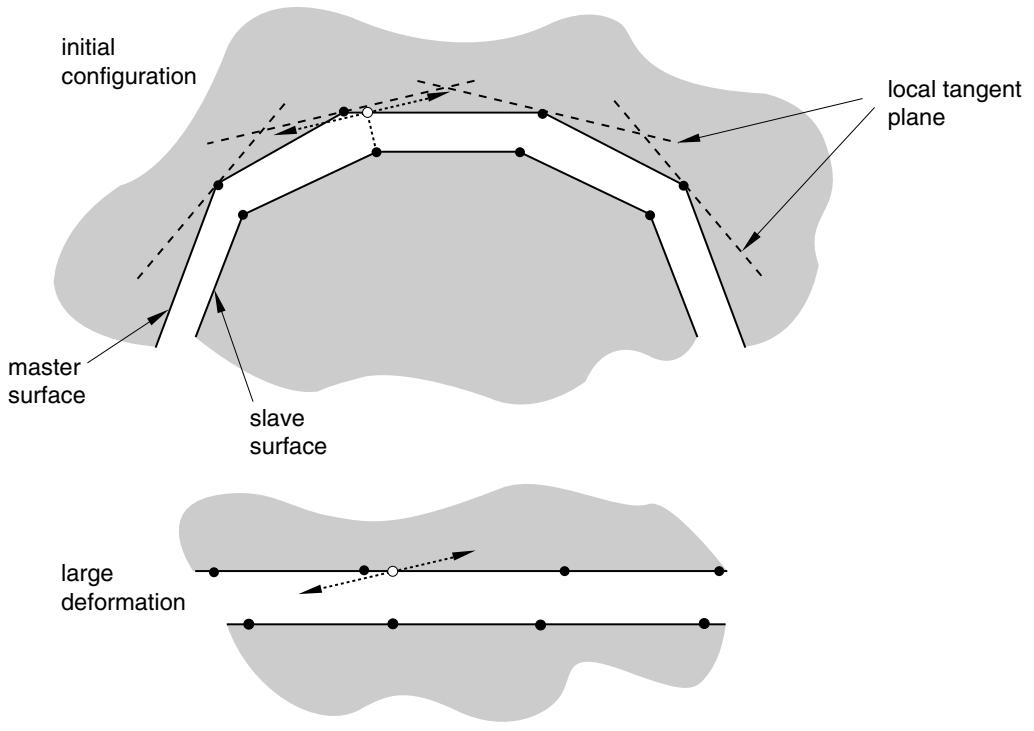The smoothly varying master surface normal and the local tangent planes that are formed with it are crucial to the success of a small-sliding analysis. As has been mentioned previously, there are several methods that can be used to modify $\mathbf { N } ( \mathbf { x } )$ ; however, they only control the initial configuration of the local tangent planes. The deformation and rotation of the master surface can reorient the local tangent planes such that they become a poor representation of the master surface. Figure 38.2.2–8 shows an example where distortion of the master surface results in such a situation. This problem can be minimized to some extent by using a more refined mesh on the master surface, thus providing more element faces to control the motion of the tangent planes. Excessive mesh refinement should not be necessary since only small sliding should occur. # Using the infinitesimal-sliding formulation The difference between the infinitesimal-sliding and small-sliding formulations is that the infinitesimalsliding formulation ignores nonlinear geometric effects. To specify the infinitesimal-sliding formulation, you choose the small-sliding contact formulation and a small-displacement formulation for the analysis step. Infinitesimal sliding assumes that both the relative motions of the surfaces and the absolute motions of the model remain small. The orientations of the local tangent planes are not updated, and the load transfer paths and the weightings assigned to each master surface node remain constant during an infinitesimal-sliding simulation. 

flowchart

```mermaid graph TD A["master surface"] --> B["slave surface"] B --> C["local tangent plane"] C --> D["initial configuration"] style A fill:#f9f,stroke:#333 style B fill:#ccf,stroke:#333 style C fill:#cfc,stroke:#333 style D fill:#fcc,stroke:#333 ```

Figure 38.2.2–8 Master surface deformation in a small-sliding contact analysis can cause problems with the local tangent planes. Input File Usage: Use both of the following options: \*STEP, NLGEOM=NO \*CONTACT PAIR, SMALL SLIDING Abaqus/CAE Usage: Interaction module: interaction editor: Sliding formulation: Small sliding Step module: step editor: Nlgeom: Off # Local tangent directions for contact Local tangent directions for contact provide a reference frame for select contact pair output variables in Abaqus/Explicit (see “Defining general contact interactions in Abaqus/Explicit,” Section 36.4.1). These local tangent directions are separate from local coordinate systems associated with user subroutines VFRIC and VUINTER. Abaqus/Explicit establishes and updates the orientation of the first local contact tangent direction, $\mathbf { t } _ { 1 }$ , at slave nodes according to the logic described below for different contact formulation types within a contact pair. The orientation of the second local tangent direction, $\mathbf { t } _ { 2 }$ , is found as the cross product of the contact normal direction, with $\mathbf { t } _ { 1 }$ . • Contact pairs not involving an analytical surface: The $\mathbf { t } _ { 1 } { \mathrm { - d i r e c t i o n } }$ at a slave node is reestablished each increment using the standard convention for calculating a first local surface tangent direction (see “Conventions,” Section 1.2.2). Local tangent directions do not co-rotate with the slave surface in this case, which is unlike general contact (see “Local tangent directions for contact” in ${ } ^ { \circ \circ } \mathrm { C }$ ontact formulation for general contact in Abaqus/Explicit,” Section 38.2.1). • Contact pairs involving an analytical surface: The $\mathbf { t } _ { 1 } { \mathrm { - d i r e c t i o n } }$ for contact is initialized at a slave node upon first contact to be aligned with the convention for the $\mathbf { t } _ { 1 }$ -direction of the analytical rigid surface discussed in “Analytical rigid surface definition,” Section 2.3.4, at the point of contact. In subsequent increments, the $\mathbf { t } _ { 1 }$ -direction for contact at a slave node evolves such that it continues to be aligned with the $\mathbf { t } _ { 1 }$ -direction of the analytical rigid surface at the current point of contact. # Contact tracking algorithms A large portion of the computational cost associated with Abaqus/Explicit contact pairs derives from the algorithms used to track the relative motion between two contacting surfaces. There are two tracking approaches for the contact pair algorithm in Abaqus/Explicit, depending on the sliding formulation that is used: finite sliding and small/infinitesimal sliding. # Finite-sliding tracking Abaqus/Explicit is designed to simulate highly nonlinear events or processes. Because it is possible for a node on one surface to contact any of the facets on the opposite surface, Abaqus/Explicit must use sophisticated search algorithms for tracking the motions of the surfaces. The contact search algorithm is designed to be robust, yet computationally efficient. This algorithm assumes that the incremental relative tangential motion between surfaces does not significantly exceed the dimensions of the master surface facets, but there is no limit to the overall relative motion between surfaces. It is rare for the incremental motion to exceed the facet size because of the small time increment used in explicit dynamic analyses. In cases involving relative surface velocities that exceed material wave speeds, it may be necessary to reduce the time increment. The contact search algorithm uses a global search at the beginning of each step, and a hierarchical global/local search algorithm is used for the other increments. The default contact search algorithm can handle the majority of typical contact situations. However, there are some situations that require special attention. We will consider a pure master-slave contact pair for discussion purposes. For a balanced master-slave contact pair, the contact search computations are performed twice for each contact pair. 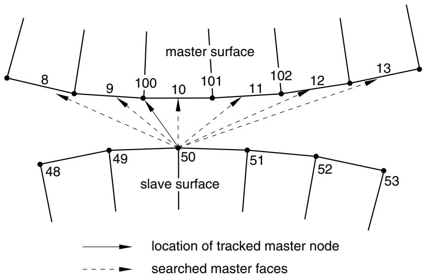# Global contact searches A global search determines the globally nearest master surface facet for each slave node in a given contact pair. A bucket sorting algorithm is used to minimize the computational expense of these searches. A two-dimensional example, without consideration of “buckets,” is shown in Figure 38.2.2–9. 

flowchart

```mermaid graph TD A["8"] --> B["9"] B --> C["100"] C --> D["10"] D --> E["101"] E --> F["11"] F --> G["102"] G --> H["12"] H --> I["13"] J["48"] --> K["49"] K --> L["50"] L --> M["51"] M --> N["52"] N --> O["53"] style A fill:#fff,stroke:#000 style B fill:#fff,stroke:#000 style C fill:#fff,stroke:#000 style D fill:#fff,stroke:#000 style E fill:#fff,stroke:#000 style F fill:#fff,stroke:#000 style G fill:#fff,stroke:#000 style H fill:#fff,stroke:#000 style I fill:#fff,stroke:#000 style J fill:#fff,stroke:#000 style K fill:#fff,stroke:#000 style L fill:#fff,stroke:#000 style M fill:#fff,stroke:#000 style N fill:#fff,stroke:#000 style O fill:#fff,stroke:#000 ```

Figure 38.2.2–9 Global search in two dimensions. The global search computes the distance from node 50 to all of the master surface facets in the same bucket as node 50. It determines that the nearest facet on the master surface to node 50 is the facet of element 10. Node 100 is the node on this facet that is nearest to node 50, and it is designated the tracked master surface node. This search is conducted for each slave node, comparing each node against all of the facets on the master surface that are in the same bucket. By default, Abaqus/Explicit performs a global search every one hundred increments for two-surface contact pairs. The frequency of the global search can be manually adjusted, as discussed in “Contact controls for contact pairs in Abaqus/Explicit,” Section 36.5.5. Despite the bucket sorting algorithm, global searches are computationally expensive: performing a global contact search in every increment will more than double the run time of many Abaqus/Explicit contact analyses. # Local contact searches Abaqus/Explicit uses a local contact search to track the motion of the surfaces during most increments of an analysis. In this approach a given slave node searches only the facets that are attached to the previously tracked master surface node. Abaqus/Explicit determines which adjacent facet is the nearest to the slave node. It then determines which node on that facet is the closest master surface node to the slave node and updates the tracked master surface node. If the closest master surface node is not the same as the previously tracked master surface node, Abaqus/Explicit performs another iteration of the local search. 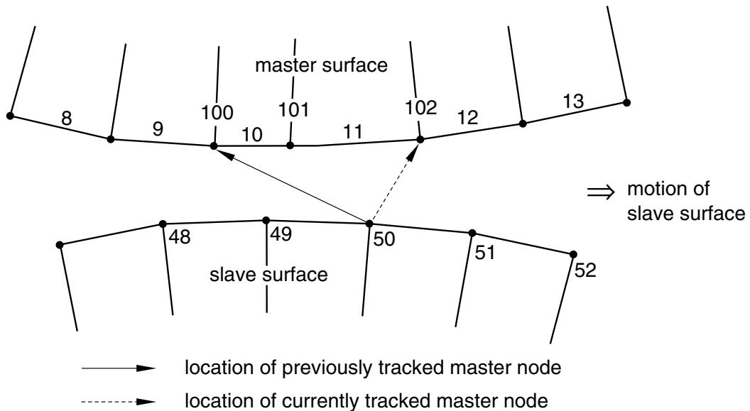In the example shown in Figure 38.2.2–10, node 50 moves as shown during an increment. In the first iteration of the search Abaqus/Explicit finds that the master surface facet on element 10 is still the closest facet of those attached to node 100 but that node 101 is now the tracked master surface node. Because the previously tracked node was node 100, Abaqus/Explicit performs another iteration. In this second iteration a new element, element 11, is found to be the closest facet and the closest master surface node is 102. Another iteration is performed because the identity of the tracked master surface node changed. In the third iteration the identity of the tracked node does not change, so Abaqus/Explicit designates node 102 as the tracked master surface node for slave node 50. A local search is substantially less expensive computationally than a global search. A slightly more expensive local search algorithm can be employed in situations where contact is not being properly enforced; this alternate algorithm is discussed in “Contact controls for contact pairs in Abaqus/Explicit,” Section 36.5.5. 

flowchart

```mermaid graph TD A["8"] --> B["9"] B --> C["100"] C --> D["101"] D --> E["11"] E --> F["102"] F --> G["12"] G --> H["13"] I["48"] --> J["49"] J --> K["50"] K --> L["51"] L --> M["52"] N["master surface"] --> O["48"] N --> P["49"] N --> Q["50"] N --> R["51"] N --> S["52"] T["→ motion of slave surface"] --> U["location of previously tracked master node"] T --> V["location of currently tracked master node"] ```

Figure 38.2.2–10 Local search in two dimensions. # Tracking approach for self-contact pairs Abaqus/Explicit uses similar contact searching methods for simulations with self-contact as for twosurface contact; however, more frequent global searches are often necessary for self-contact problems. By default, contact pairs with self-contact use a global contact search every four increments, compared to every 100 increments for two-surface contact pairs; the frequency of the global searches can be manually adjusted (see “Contact controls for contact pairs in Abaqus/Explicit,” Section 36.5.5). If several facets that are unconnected to each other are found to be near a slave node during global tracking, global tracking automatically will be performed more frequently than the specified number of increments. Despite this precaution, the self-contact algorithm will be less robust if you specify a search frequency that is significantly lower than the default. # Small-sliding (or infinitesimal-sliding) tracking approach When the small-sliding or infinitesimal-sliding contact approach is invoked (see “Sliding formulation” in “Contact formulations for contact pairs in Abaqus/Explicit,” Section 38.2.2), Abaqus/Explicit performs a single global search at the beginning of the first step to determine the globally nearest master surface facet for each slave node in the given contact pair. Once the nearest facet has been determined, the nearest point on that facet defines the anchor point. Contact constraints will not be applied to slave nodes that do not project onto any master surface facet. No further tracking is performed during the step or for subsequent steps in which the contact pair remains active. This makes the small-sliding/infinitesimal-sliding contact approach less expensive computationally than the finite-sliding contact approach. The cost savings are most significant for three-dimensional contact problems. # 38.2.3 CONTACT CONSTRAINT ENFORCEMENT METHODS IN Abaqus/Explicit Products: Abaqus/Explicit Abaqus/CAE # References • “Defining general contact interactions in Abaqus/Explicit,” Section 36.4.1 • “Defining contact pairs in Abaqus/Explicit,” Section 36.5.1 • \*CONTACT • \*CONTACT PAIR • “Specifying master-slave assignments for general contact,” Section 15.13.6 of the Abaqus/CAE User’s Guide, in the HTML version of this guide # Overview Abaqus/Explicit uses two different methods to enforce contact constraints: • The kinematic contact algorithm uses a kinematic predictor/corrector contact algorithm to strictly enforce contact constraints (for example, no penetrations are allowed). • The penalty contact algorithm has a weaker enforcement of contact constraints but allows for treatment of more general types of contact. Contact pairs in Abaqus/Explicit use kinematic enforcement by default, but penalty enforcement can be specified for individual contact pairs. General contact always uses penalty enforcement. Both methods conserve momentum between the contacting bodies. # Kinematic contact algorithm A summary of the default kinematic algorithm that Abaqus/Explicit uses to enforce contact with the contact pair algorithm is presented below. It is a predictor/corrector algorithm and, therefore, has no influence on the stable time increment. It is easier to describe the algorithm by first considering a pure master-slave contact pair. # Kinematic enforcement of contact conditions in a pure master-slave contact pair In this case in each increment of the analysis Abaqus/Explicit first advances the kinematic state of the model into a predicted configuration without considering the contact conditions. Abaqus/Explicit then determines which slave nodes in the predicted configuration penetrate the master surfaces. The depth of each slave node’s penetration, the mass associated with it, and the time increment are used to calculate the resisting force required to oppose penetration. For hard contact, this is the force which, had it been applied during the increment, would have caused the slave node to exactly contact the master surface. The next step depends on the type of master surface used. • When the master surface is formed by element faces, the resisting forces of all the slave nodes are distributed to the nodes on the master surface. The mass of each contacting slave node is also distributed to the master surface nodes and added to their mass to determine the total inertial mass of the contacting interfaces. Abaqus/Explicit uses these distributed forces and masses to calculate an acceleration correction for the master surface nodes. Acceleration corrections for the slave nodes are then determined using the predicted penetration for each node, the time increment, and the acceleration corrections for the master surface nodes. Abaqus/Explicit uses these acceleration corrections to obtain a corrected configuration in which the contact constraints are enforced. • In the case of an analytical rigid master surface, the resisting forces of all slave nodes are applied as generalized forces on the associated rigid body. The mass of each contacting slave node is added to the rigid body to determine the total inertial mass of the contacting interfaces. The generalized forces and added masses are used to calculate an acceleration correction for the analytical rigid master surface. Acceleration corrections for the slave nodes are then determined by the corrected motion of the master surface. 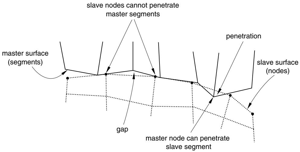When using hard kinematic contact, it is still possible with the pure master-slave algorithm for the master surface to penetrate the slave surface in the corrected configuration (see Figure 38.2.3–1). 

flowchart

```mermaid graph TD A["master surface (segments)"] --> B["slave nodes cannot penetrate master segments"] B --> C["penetration"] C --> D["slave surface (nodes)"] D --> E["master node can penetrate slave segment"] E --> F["gap"] F --> A ```

Figure 38.2.3–1 Master surface penetrations into the slave surface of a pure master-slave contact pair due to coarse discretization. Using a sufficiently refined mesh on the slave surface will minimize such penetrations. Softened kinematic contact will allow penetrations since corrections are made to satisfy the pressure-overclosure relationship at the slave-nodes, not the condition of zero penetration.