# 40.1.1 CONTACT MODELING WITH ELEMENTS
Abaqus/Standard offers a variety of contact elements that can be used when contact between two bodies cannot be simulated with the surface-based contact approach (Chapter 36, “Defining Contact Interactions”). These elements include the following:
• Gap contact elements: Mechanical and thermal contact between two nodes is modeled with gap elements (“Gap contact elements,” Section 40.2.1). For example, these elements can be used to model the contact between a piping system and its supports. They can also be used to model an inextensible cable that supports only tensile loads.
• Tube-to-tube contact elements: Contact between two pipes or tubes is modeled using tube-to-tube contact elements (“Tube-to-tube contact elements,” Section 40.3.1) in conjunction with slide lines. These elements can, for example, be used to simulate the process of running tubular components into an oil well (drill rod or J-tube analysis). They might also be used to simulate a catheter being inserted into a blood vessel.
• Slide line contact elements: Finite-sliding contact between two axisymmetric structures that may undergo asymmetric deformations can be modeled using slide line contact elements (“Slide line contact elements,” Section 40.4.1) in conjunction with user-defined slide lines. Slide line elements can, for example, be used to model threaded connectors.
• Rigid surface contact elements: Contact between an analytical rigid surface and an axisymmetric deformable body that may undergo asymmetric deformations can be modeled with rigid surface contact elements (“Rigid surface contact elements,” Section 40.5.1). For example, rigid surface contact elements might be used to model the contact between a rubber seal and a much stiffer structure.
# 40.2 Gap contact elements
• “Gap contact elements,” Section 40.2.1
• “Gap element library,” Section 40.2.2
# 40.2.1 GAP CONTACT ELEMENTS
Product: Abaqus/Standard
# References
• “Gap element library,” Section 40.2.2
• \*GAP
# Overview
Gap elements:
• allow for contact between two nodes;
• allow for the nodes to be in contact (gap closed) or separated (gap open) with respect to particular directions and separation conditions;
• are always defined in three dimensions but can also be used in two-dimensional and axisymmetric models;
• allow contact to be defined on any type of element, including substructures and user-defined elements;
• can be used to model contact in fixed or rotating directions;
• can be used to model node-to-node contact and thermal interactions in a fixed direction in space in coupled temperature-displacement simulations; and
• can be used to model node-to-node thermal interactions in heat transfer analyses.
A general discussion of contact modeling in Abaqus/Standard can be found in Chapter 36, “Defining Contact Interactions.”
# Choosing and defining a gap element
GAPUNI elements model contact between two nodes when the contact direction is fixed in space. GAPCYL elements model contact between two nodes when the contact direction is orthogonal to an axis. GAPSPHER elements model contact between two nodes when the contact direction is arbitrary in space. GAPUNIT elements model contact and thermal interactions between two nodes when the contact direction is fixed in space. DGAP elements model thermal interactions between two nodes in heat transfer analysis.
Gap elements are defined by specifying the two nodes forming the gap and providing geometric data defining the initial state and, if necessary, the direction of the gap.
# Defining the gap element’s properties
You must associate the gap behavior with a set of gap elements.
Input File Usage: \*GAP, ELSET=element\_set\_name
# GAPUNI and GAPUNIT elements
The contact behavior of the interface being modeled with GAPUNI and GAPUNIT elements is defined by the initial separation distance (clearance), $d ,$ of the gap and the contact direction, . In addition, GAPUNIT elements have temperature degrees of freedom that allow modeling of thermal interactions in coupled temperature-displacement analyses.
# Clearance between GAPUNI nodes
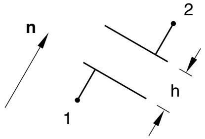
Abaqus/Standard defines the current clearance between two nodes of the gap, $h ,$ a s
$$
h = d + \mathbf {n} \cdot (\mathbf {u} ^ {2} - \mathbf {u} ^ {1}),
$$
where ${ \bf u } ^ { 1 }$ and ${ \bf u } ^ { 2 }$ are the total displacements at the first and the second node forming the GAPUNI element. Figure 40.2.1–1 shows the configuration of the GAPUNI element. When h becomes negative, the gap contact element is closed and the constraint $h = 0$ is imposed.
text_image
n
1
2
h
$$
\mathsf {h} = \mathsf {d} + \mathsf {n} \cdot (\mathsf {u} ^ {2} - \mathsf {u} ^ {1}) \geq 0
$$
Figure 40.2.1–1 GAPUNI and GAPUNIT contact elements.
You specify a value for d. If you provide a positive value, the gap is open initially. If $\scriptstyle d = 0 ,$ , the gap is initially closed. If d is negative, the gap is considered overclosed at the start of the analysis and an initial interference fit problem is defined. Details about modeling interference fit problems with gap elements are discussed below.
Input File Usage: \*GAP d
# Specifying the contact direction
You can specify the contact direction. Otherwise, Abaqus/Standard will calculate the gap direction, , by using the initial positions of the two nodes forming the element, $\mathbf { X } ^ { 1 }$ and $\mathbf { X } ^ { 2 }$ :
$$
\mathbf {n} = \left(\mathbf {X} ^ {2} - \mathbf {X} ^ {1}\right) / \left| \mathbf {X} ^ {2} - \mathbf {X} ^ {1} \right|.
$$
An error message is issued if $\mathbf { X } ^ { 2 } = \mathbf { X } ^ { 1 }$ (if the two gap element nodes have the same initial coordinates). In this situation you must define . The normal usually points from the first node of the element to the second, unless the gap is overclosed at the start of the analysis. In that case specify so that the correct contact direction is used for the gap element.
If you specify the gap direction rather than allowing Abaqus/Standard to calculate it, the contact calculations consider only , the displacements of the gap element’s nodes, and the ordering of the nodes in the element definition: the initial coordinates of the nodes play no role in the calculations.
The orientation of does not change during the analysis.
Input File Usage: \*GAP
, X-direction cosine, Y-direction cosine, Z-direction cosine
Local basis system for GAPUNI element output
Abaqus/Standard reports the pressure transmitted across the gap and the shear stresses that are orthogonal to the contact direction as element output for GAPUNI elements. You must supply the contact area associated with these elements for Abaqus/Standard to compute the pressure and the shear stress values. It also reports the current clearance in the gap, h, and the relative motions of the GAPUNI nodes orthogonal to the contact direction. The relative motions and the shear stresses are reported in local surface directions that are formed using the standard Abaqus convention for defining directions on surfaces in space (see “Conventions,” Section 1.2.2). The contact direction defines a surface in space on which the local axes are formed.
Input File Usage: \*GAP
$, \ , \ , \ c r o s s - s e c t i o n a l \ a r e a$
# GAPCYL elements
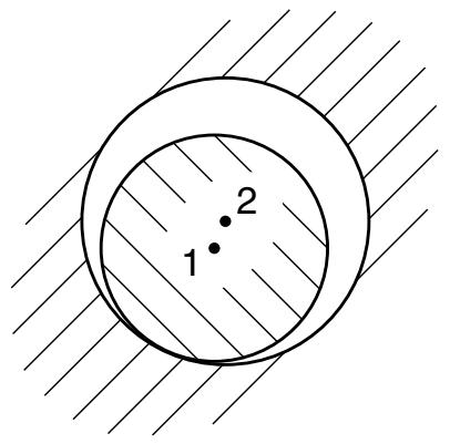
GAPCYL elements can be used to model two very different contact situations: contact between two rigid tubes, where the smaller one is inside the larger tube, and contact between two rigid tubes along their external surfaces. Both cases are shown in Figure 40.2.1–2.
The behavior of a GAPCYL element is defined by the initial separation distance between the nodes, d; the current positions of the element’s node; and the axis of the GAPCYL element. The axis of the GAPCYL element defines the plane in which the contact direction, , lies. You specify d and the direction cosines of the GAPCYL element axis.
The value is not allowed: it would enforce the distance between the nodes to be exactly zero at all times, which does not correspond to a contact problem.
Input File Usage: \*GAP
d, X-direction cosine, Y-direction cosine, Z-direction cosine
Defining the gap clearance for Case 1 (when d is positive)
If d is positive, the GAPCYL element models contact between two rigid tubes of different diameter, where the smaller tube is located inside the larger tube (see Case 1 in Figure 40.2.1–2). In this case d is the maximum allowable separation. Each tube is represented by a node on its axis, with the axes connected by the GAPCYL element; and d corresponds to the difference between the radii of the tubes.
text_image
1
2
$\mathsf { C a s e \ 1 } \quad \mathsf { d } = \mathsf { r } _ { 2 } - \mathsf { r } _ { 1 }$
$$
h = d - \left| \overline {{{\mathbf {x}}}} ^ {2} - \overline {{{\mathbf {x}}}} ^ {1} \right| \geq 0
$$
text_image
1
2
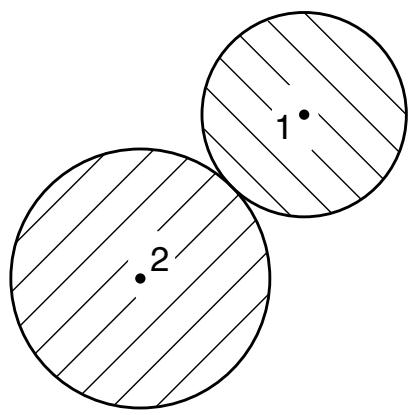
$\begin{array} { r l } { \mathsf { C a s e 2 } } & { { } \mathsf { d } = - \left( \mathsf { r } _ { 1 } + \mathsf { r } _ { 2 } \right) } \end{array}$
$$
h = \left| \overline {{{\mathbf {x}}}} ^ {2} - \overline {{{\mathbf {x}}}} ^ {1} \right| - | d | \geq 0
$$
Figure 40.2.1–2 Gap clearance for GAPCYL/GAPSPHER contact elements.
The gap between the tubes closes when the two nodes become separated by more than d in any direction in the plane defined by the axis of the GAPCYL element.
Abaqus/Standard defines the current gap opening, h, in GAPCYL elements for Case 1 as
$$
h = d - | \overline {{\mathbf {x}}} ^ {2} - \overline {{\mathbf {x}}} ^ {1} | \qquad \mathrm{with} \qquad \overline {{\mathbf {x}}} ^ {N} = \mathbf {x} ^ {N} - \mathbf {a} \left(\mathbf {a} \cdot \mathbf {x} ^ {N}\right),
$$
where $\mathbf { x } ^ { N }$ is the current position of node N, d is the specified initial separation, and a is the axis of the GAPCYL element.
If the initial position of the tube axes is such that the distance between them is less than $d ,$ the GAPCYL element is open initially. If the distance is equal to $d ,$ the element is closed initially; and if the distance is greater than $d ,$ an initial overclosure (interference) is defined. Details about modeling interference fit problems with gap elements are discussed below.
# Defining the gap clearance for Case 2 (when d is negative)
If d is negative, the GAPCYL element models external contact between two parallel rigid cylinders (see Case 2 in Figure 40.2.1–2). In this case $d |$ is the minimum allowable separation of the nodes. Each cylinder is represented by a node on its axis connected by the GAPCYL element, and $d |$ corresponds to the sum of the radii of the cylinders. The gap closes when the two nodes approach each other to within $d |$ in any direction in the plane defined by the axis of the GAPCYL element.
Abaqus/Standard defines the current gap opening, $h ,$ in GAPCYL elements for Case 2 as
$$
h = \left| \overline {{{\mathbf {x}}}} ^ {2} - \overline {{{\mathbf {x}}}} ^ {1} \right| - | d | \qquad \mathrm{with} \qquad \overline {{{\mathbf {x}}}} ^ {N} = \mathbf {x} ^ {N} - \mathbf {a} \left(\mathbf {a} \cdot \mathbf {x} ^ {N}\right).
$$
If the initial position of the cylinder axes is such that the distance between them is greater than , the GAPCYL element is open initially. If the distance is equal to , the element is closed initially; and if the distance is less than , an initial overclosure (interference) is defined. Details about modeling interference fit problems with gap elements are discussed below.
# Local basis system for GAPCYL element output
Abaqus/Standard reports the pressure transmitted across the gap and the shear stresses that are orthogonal to the contact direction as element output for GAPCYL elements. You must supply the contact area associated with these elements for Abaqus/Standard to compute the pressure and the shear stress values. It also reports the current clearance in the gap, h, and the relative motions of the element’s nodes that are orthogonal to the contact direction. The relative motions and the shear stresses are reported in local surface directions that are formed using the standard Abaqus convention for defining directions on surfaces in space (see “Conventions,” Section 1.2.2). The contact direction defines a surface in space on which the local axes are formed, and the slip is calculated from the relative motions in the surface directions.
Abaqus/Standard updates the contact direction for GAPCYL elements based on the motion of the nodes forming the elements. However, the orientation of is not updated during the analysis.
Input File Usage: $\ast \mathrm { G A P }$ , , , , cross-sectional area
# GAPSPHER elements
GAPSPHER elements can be used to model two very different contact situations: contact between two rigid spheres where the smaller sphere is inside the larger, hollow sphere, and contact between two rigid spheres along their external surfaces. Both cases are shown in Figure 40.2.1–2.
The behavior of a GAPSPHER element is defined by the minimum or maximum separation distance between the nodes, d, and the current positions of the element’s nodes. You specify the minimum or maximum separation distance, d. The contact direction is defined by the current position of the nodes.
The value is not allowed: it would enforce the distance between the nodes to be exactly zero at all times, which does not correspond to a contact problem.
Input File Usage: \*GAP d
# Defining the gap clearance for Case 1 (when d is positive)
If d is positive, the GAPSPHER element models contact between a rigid sphere inside another (larger) hollow rigid sphere (see Case 1 in Figure 40.2.1–2). In this case d is the maximum allowable separation of the nodes forming the gap. Each sphere is represented by a node at its center, with the centers connected by the GAPSPHER element; and d corresponds to the difference between the radii of the spheres. The gap closes when the two nodes become separated by more than d.
Abaqus/Standard defines the current gap opening, h, for Case 1 as
$$
h = d - \left| \mathbf {x} ^ {2} - \mathbf {x} ^ {1} \right|,
$$
with $\mathbf { x } ^ { N }$ the current position of node N and d the specified separation.
If the initial position of the tube axes is such that the distance between them is less than $d ,$ the GAPSPHER element is open initially. If the distance is equal to $d ,$ the element is closed initially; and if the distance is greater than $d ,$ an initial overclosure (interference) is defined. Details about modeling interference fit problems with gap elements are discussed below.
Defining the gap clearance for Case 2 (when d is negative)
If d is negative, the GAPSPHER element models external contact between two rigid spheres (see Case 2 in Figure 40.2.1–2). In this case $d |$ is the minimum allowable separation of the nodes forming the gap. Each sphere is represented by a node at its center connected by the GAPSPHER element; and $d |$ corresponds to the sum of the radii of the spheres. The gap closes when the two nodes approach each other to within $d |$ .
Abaqus/Standard defines the current gap opening, $h ,$ for Case 2 as
$$
h = \left| \mathbf {x} ^ {2} - \mathbf {x} ^ {1} \right| - | d |.
$$
If the initial position of the cylinder axes is such that the distance between them is greater than $d | _ { i }$ , the GAPSPHER element is open initially. If the distance is equal to $d | ,$ , the element is closed initially; and if the distance is less than $d |$ , an initial overclosure (interference) is defined. Details about modeling interference fit problems with gap elements are discussed below.
Local basis system for GAPSPHER element output
Abaqus/Standard reports the pressure transmitted across the gap and the shear stresses that are orthogonal to the contact direction as element output for GAPSPHER elements. You must supply the contact area associated with these elements for Abaqus/Standard to compute the pressure and the shear stress values. It also reports the current clearance in the gap, h, and the relative motions of the element’s node that are orthogonal to the contact direction. The relative motions and the shear stresses are reported in local surface directions that are formed using the standard Abaqus convention for defining directions on surfaces in space; see “Conventions,” Section 1.2.2. The contact direction defines a surface in space on which the local axes are formed, and the slip is calculated from the relative motions in the surface directions.
Abaqus/Standard updates the contact direction for GAPSPHER elements based on the motion of the nodes forming the elements.
Input File Usage: \*GAP
$, \ , \ , \ c r o s s - s e c t i o n a l \ a r e a$