the other hand, in the analysis of the arch, the precollapse displacements are large and the linearized buckling analysis very much overestimates the collapse load unless the state of loading corresponding to $\Delta t$ is already close to that load. In general, a linearized buckling analysis will give good results if the structure displays a column type of buckling behavior. However, as mentioned already, even if the linearized buckling load cannot be used as an estimate of the actual collapse load of the structure, it may be important to impose the buckling mode as an imperfection on the structural model. This imperfection may well be present in the actual physical structure and, if the effect is significant, should be included in the analysis. 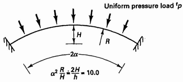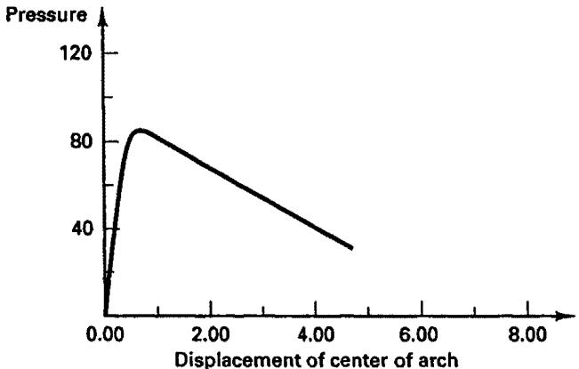To illustrate these thoughts, consider the analysis of the arch in Fig. 6.23. The complete structure is modeled using ten two-node isoparametric beam elements. In the analysis, 

text_image

Uniform pressure load ^t p H R 2α α² R/H ÷ 2H/h = 10.0

R = 64.85 $\alpha = 22.5^{\circ}$ $E = 2.1 \times 10^{6}$ $\nu = 0.3$ h=b=1.0 Cross section:  (a) Arch considered; ten 2-node isoparametric beam elements are used to model the complete structure 

line

| Displacement of center of arch | Pressure | | ----------------------------- | -------- | | 0.00 | 0.00 | | 1.00 | 110.00 | | 2.00 | 100.00 | | 3.00 | 80.00 | | 4.00 | 60.00 | | 5.00 | 40.00 | | 6.00 | 30.00 | | 7.00 | 35.00 | | 8.00 | 40.00 |

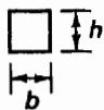
(b) Displacement response of perfectly symmetric structure Figure 6.23 Collapse analysis of arch 

line

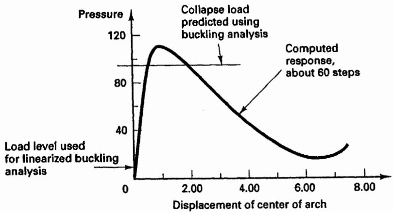
| Mode | p_cr | | ------------- | ---- | | First mode | 95 | | Second mode | 150 |

(c) Collapse loads and buckling modes using a linearized buckling analysis ( $\Delta^{f}p = 10$ ) 

line

| Displacement of center of arch | Pressure | | ------------------------------ | -------- | | 0.00 | 0 | | 0.50 | 80 | | 4.50 | 35 |

(d) Response of arch with antisymmetric imperfection Figure 6.23 (continued) symmetry conditions were not used so as to allow antisymmetric behavior of the model. The objective was to predict the collapse and postcollapse response. Figure 6.23(b) shows the response calculated using a load-displacement-constraint method as described in Section 8.4.3. Also, a linearized buckling analysis was performed using as state $t - \Delta t$ the unstressed configuration and as state $\Delta t$ the configuration corresponding to a pressure of 10. The two smallest critical pressures and corresponding buckling modes are shown in Fig. 6.23(c). We note that the smallest critical pressure corresponds to an antisymmetric buckling displacement. However, the response in Fig. 6.23(b) was obtained assuming a perfectly symmetric arch, and hence symmetric deformations were calculated in each solution step. The antisymmetric linearized buckling deformations indicate that the structure is sensitive to antisymmetric imperfections. Hence, we introduced a geometric imperfection into the model of the arch by adding a multiple of the first buckling mode, $\phi_{1}$ , to the geometry of the undeformed arch. In this addition the mode is scaled so that the magnitude of the imperfection is less than 0.01 (one-hundredth of the cross-sectional depth). Figure 6.23(d) shows the calculated response—again using a load-displacement-constraint method as discussed in Section 8.4.3—of the arch with this geometric imperfection. We notice that the collapse load now predicted is significantly smaller than the value given in Fig. 6.23(b). This reduction in the collapse load is associated with a nonsymmetric behavior of the structural model which is made possible because of the imposed geometric imperfection. The collapse analysis of a structure requires, in general, an incremental load analysis, which should include the geometric and material nonlinearities. The preceding discussion indicates that structural imperfections can also have a major effect on the predicted load-carrying capacity of a structure. Hence, when such a situation is anticipated, imperfections should be introduced in the structural model. Here we considered geometric imperfections and a simple example. In the analysis of a complex structure, multiples of the 2nd, 3rd, . . . buckling modes would also be added to the geometry, but it may also be appropriate to introduce perturbations in the material properties or the applied loading, all of which should serve to excite the structure to embark on the deformation path that corresponds to the smallest load-carrying capacity. While we have presented in this chapter the formulation of the incremental equations, the solution of these equations and the solution of the buckling eigenproblem are discussed in Chapters 8 and 11, respectively. 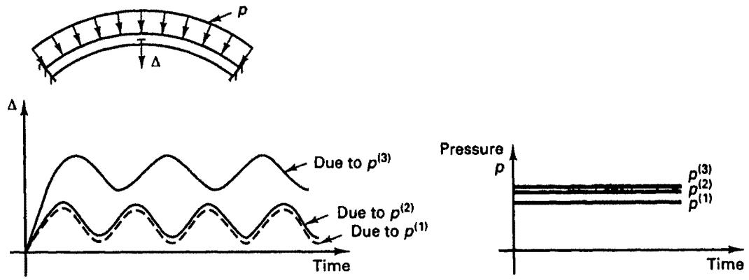Finally, we should mention that in addition to the static buckling analyses, dynamic solutions also may need to be considered. A dynamic buckling or collapse analysis requires that complete dynamic incremental analyses be performed for given different load levels (including of course the possible effects of imperfections). Figure 6.24 illustrates a sequence of such analyses. The structural model is stable for the pressure levels $p^{(1)}$ and $p^{(2)}$ but is unstable for the load level $p^{(3)}$ . If the difference between $p^{(2)}$ and $p^{(3)}$ is small, a good estimate of the collapse load is given by $p^{(2)}$ , otherwise further analyses are needed to decrease the difference between the load level at which the structure is still stable and the level at which it is unstable. Such dynamic solutions are obtained using the procedures described in Chapter 9. # 6.8.3 The Effects of Element Distortions We mentioned in Sections 5.3.3 and 5.5.5 that finite elements are in general most effective in the prediction of displacements and stresses when they are undistorted. However, in practice, elements must largely be of general straight-sided shapes with angular distortions 

text_image

p Δ Δ Due to p^(3) Due to p^(2) Due to p^(1) Time Pressure p p^(3) p^(2) p^(1) Time

Figure 6.24 Dynamic buckling of arch; the structure shows a stable dynamic response due to load levels $p^{(1)}$ and $p^{(2)}$ and a much larger response due to $p^{(3)}$ . (for example, we use general quadrilateral elements in two-dimensional analysis) in order to provide mesh gradings and to mesh complex geometries effectively. To model curved boundaries, curved element sides or faces also need to be used. In addition, in geometric nonlinear analysis, significant angular and curved edge distortions and distortions due to movement of noncorner element nodes may arise as a consequence of the deformations. While the actual solution error increases as a result of all these element distortions, as long as the distortions are “small” (as discussed in Section 5.3.3), the order of convergence is not affected. We also noted that frequently the Lagrangian elements are more effective than the elements lacking the interior nodes. Using the large displacement formulations, the principle of virtual displacements is applied to each individual element corresponding to the current configuration instead of the initial configuration used in linear analysis. Thus, element distortions must be expected to affect the accuracy of the nonlinear response prediction in a manner similar to that in linear analysis, but now the considerations concerning the element distortions in linear analysis summarized in Section 5.3.3 are applicable throughout the response history of the mesh. In an analysis it is therefore necessary to monitor the changing shape of each element, and if element distortions adversely affect the response prediction, a different and finer mesh may be required for the geometrically nonlinear analysis. Also, mesh rezoning can be used at certain critical times with the objective to keep closely to an element layout in which only the angular distortions are present. In these mesh constructions Lagrangian elements are used very effectively (see N. S. Lee and K. J. Bathe [A, B]). We should also point out that these considerations are equally applicable to the TL and the UL formulations because, except for certain constitutive assumptions, both formulations are completely equivalent (see Example 6.23). # 6.8.4 The Effects of Order of Numerical Integration To select the appropriate numerical integration scheme and order of integration in nonlinear analysis, some specific considerations beyond those already discussed in Section 5.5.5 are important. Based on the information given above and in Section 5.5.5 on the required integration order for undistorted and distorted elements, we can directly conclude that in geometric nonlinear analysis, at least the same integration order should be employed as in linear analysis. However, a higher integration order than that used in linear analysis may be required in the analysis of materially nonlinear response simply in order for the analysis to capture the onset and spread of the materially nonlinear conditions accurately enough. Specifically, since the material nonlinearities are measured only at the integration points of the elements, the use of a relatively low integration order may mean that the spread of the materially nonlinear conditions through the elements is not represented accurately. This consideration is particularly important in the materially nonlinear analysis of beam, plate, and shell structures and also leads to the conclusion that the Newton-Cotes methods may be effective (say for integration in certain directions) because then integration points for stiffness and stress evaluations are on the boundaries of the elements (e.g., on the top and bottom surfaces of a shell).  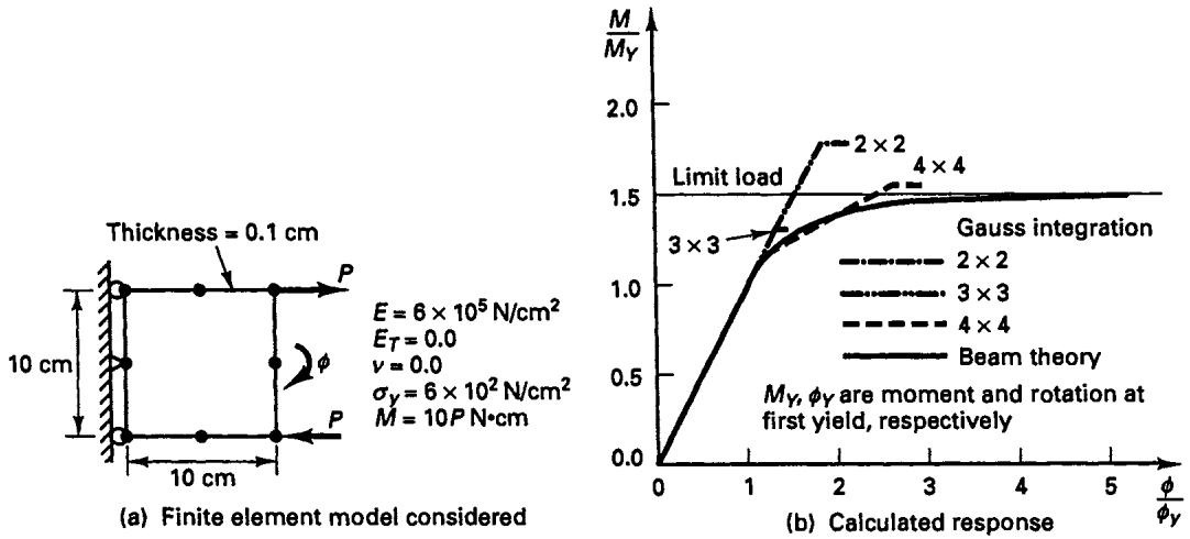Figure 6.25 Effect of integration order in elastic-plastic analysis of beam section Figure 6.25 gives the results of using different orders of Gauss integration for an eight-node plane stress element representing the section of a beam. The element is subjected to an increasing bending moment, and the numerically predicted response is compared with the response calculated using beam theory. This analysis illustrates that to predict the materially nonlinear response accurately a higher integration order in the thickness direction of the beam is required than in linear analysis. Another example that demonstrates the effect of using different integration orders in materially nonlinear analysis follows. 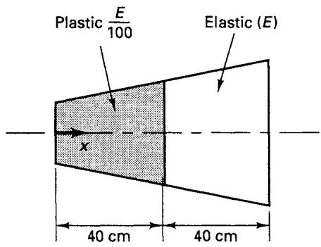EXAMPLE 6.27: Consider element 2 in Example 4.5 and assume that in an elastoplastic analysis the stresses at time t in the element are such that the tangent moduli of the material are equal to E/100 for $0 \leq x \leq 40$ and equal to E for $40 < x \leq 80$ as illustrated in Fig. E6.27. Evaluate the tangent stiffness matrix 'K using one-, two-, three-, and four-point Gauss integration and compare these results with the exact stiffness matrix. Consider only material nonlinearities. 

text_image

Plastic E/100 Elastic (E) 40 cm 40 cm

Figure E6.27 Element 2 of Example 4.5 in elastic-plastic conditions For the evaluation of the matrix 'K we use the information given in Example 4.5 and in Table 5.6. Thus, we obtain the following results: One-point integration: $$ { } ^ { t } \mathbf { K } = 2 \times 4 0 \left[ \begin{array} { c } - \frac { 1 } { 8 0 } \\ \frac { 1 } { 8 0 } \end{array} \right] \frac { E } { 1 0 0 } \left[ \begin{array} { c c } - \frac { 1 } { 8 0 } & \frac { 1 } { 8 0 } \end{array} \right] ( 1 + 1 ) ^ { 2 } = 0 . 0 0 0 5 E \left[ \begin{array} { c c } 1 & - 1 \\ - 1 & 1 \end{array} \right] $$ Two-point integration: $$ ^ {t} \mathbf {K} = 1 \times 4 0 \left[ \begin{array}{c} - \frac {1}{8 0} \\ \frac {1}{8 0} \end{array} \right] \frac {E}{1 0 0} \left[ \begin{array}{c c} - \frac {1}{8 0} & \frac {1}{8 0} \end{array} \right] \left(1 + 1 - \frac {1}{\sqrt {3}}\right) ^ {2} $$ $$ + 1 \times 4 0 \left[ \begin{array}{c} - \frac {1}{8 0} \\ \frac {1}{8 0} \end{array} \right] E \left[ \begin{array}{c c} - \frac {1}{8 0} & \frac {1}{8 0} \end{array} \right] \left(1 + 1 + \frac {1}{\sqrt {3}}\right) ^ {2} $$ $$ = 0. 0 4 1 6 4 E \left[ \begin{array}{c c} 1 & - 1 \\ - 1 & 1 \end{array} \right] $$ Three-point integration: $$ ^ {t} \mathbf {K} = \frac {5}{9} 4 0 \left[ \begin{array}{c} - \frac {1}{8 0} \\ \frac {1}{8 0} \end{array} \right] \frac {E}{1 0 0} \left[ \begin{array}{c c} - \frac {1}{8 0} & \frac {1}{8 0} \end{array} \right] \left(1 + 1 - \frac {\sqrt {3}}{5}\right) ^ {2} $$ $$ + \frac {8}{9} 4 0 \left[ \begin{array}{c} - \frac {1}{8 0} \\ \frac {1}{8 0} \end{array} \right] \frac {E}{1 0 0} \left[ \begin{array}{c c} - \frac {1}{8 0} & \frac {1}{8 0} \end{array} \right] (1 + 1) ^ {2} $$ $$ + \frac {5}{9} 4 0 \left[ \begin{array}{c} - \frac {1}{8 0} \\ \frac {1}{8 0} \end{array} \right] E \left[ \begin{array}{c c} - \frac {1}{8 0} & \frac {1}{8 0} \end{array} \right] (1 + 1 + \sqrt {3} / 5) ^ {2} $$ $$ \mathbf {K} = 0. 0 2 7 0 0 E \left[ \begin{array}{c c} 1 & - 1 \\ - 1 & 1 \end{array} \right] $$ Four-point integration: $$ n = 4 \quad \begin{array}{l l} r _ {i} & \alpha_ {i} \\ \pm 0. 8 6 1 1 \dots & 0. 3 4 7 8 \dots \\ \pm 0. 3 3 9 9 \dots & 0. 6 5 2 1 \dots \end{array} $$ $$ ^ {t} \mathbf {K} = 0. 3 4 7 8 \dots (4 0) \left[ \begin{array}{c} - \frac {1}{8 0} \\ \frac {1}{8 0} \end{array} \right] \frac {E}{1 0 0} \left[ \begin{array}{c c} - \frac {1}{8 0} & \frac {1}{8 0} \end{array} \right] (1 + 1 - 0. 8 6 1 1 \dots) ^ {2} $$ $$ + \dots $$ $$ ^ {\prime} \mathbf {K} = 0. 0 4 0 2 6 E \left[ \begin{array}{c c} 1 & - 1 \\ - 1 & 1 \end{array} \right] $$ The exact stiffness matrix is $$ \begin{array}{l} \mathbf {K} = \left[ \begin{array}{c} - \frac {1}{8 0} \\ \frac {1}{8 0} \end{array} \right] \frac {E}{1 0 0} \left[ \begin{array}{l l} - \frac {1}{8 0} & \frac {1}{8 0} \end{array} \right] \left\{\int_ {0} ^ {4 0} \left(1 + \frac {y}{4 0}\right) ^ {2} d y + \int_ {4 0} ^ {8 0} 1 0 0 \left(1 + \frac {y}{4 0}\right) ^ {2} d y \right\} \\ = \left[ \begin{array}{c} - \frac {1}{8 0} \\ \frac {1}{8 0} \end{array} \right] E \left[ \begin{array}{l l} - \frac {1}{8 0} & \frac {1}{8 0} \end{array} \right] \left\{\frac {4 0}{3 0 0} \left(1 + \frac {y}{4 0}\right) ^ {3} \right| _ {0} ^ {4 0} + \frac {4 0}{3} \left(1 + \frac {y}{4 0}\right) ^ {3} \left| _ {4 0} ^ {8 0} \right\} \\ ^ {\prime} \mathbf {K} = 0. 0 3 9 7 3 E \left[ \begin{array}{c c} 1 & - 1 \\ - 1 & 1 \end{array} \right] \\ \end{array} $$ It is interesting to note that in this case the two-point integration yields more accurate results than the three-point integration and that a good approximation to the exact stiffness matrix is obtained using four-point integration. The above remarks show that in nonlinear analysis the use of a higher integration order than in linear analysis may be appropriate. Such higher integration order, when needed, should of course be used for displacement-based and mixed finite elements. Hence, referring to Section 5.5.6, where we briefly mentioned the use of reduced and selective integration, our recommendations given in that section also pertain to, and are at least equally important in, nonlinear analysis. In short, the recommendations were that only well-formulated displacement-based and mixed elements should be used. To calculate the element matrices of a mixed formulation effectively, in some special cases a displacement-based formulation with a special integration scheme can be used. We should, however, note that this correspondence may hold only in linear analysis, and it is important that the correspondence be studied for nonlinear analysis in each individual case. 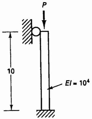# 6.8.5 Exercises 6.95. Use a computer program to calculate the linearized buckling load of the column structure shown. Compare your calculated results with an analytical solution. (Hint: Here you can use Hermitian beam elements, isoparametric beam elements, or plane stress elements to model the column.) 

text_image

P 10 EI = 10^4

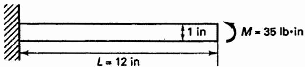
6.96. Use a computer program to calculate the large displacement response of the cantilever beam shown. Compare your results with an analytical solution (see, for example, J. T. Holden [A]). 

text_image

1 in M = 35 lb·in L = 12 in

Thickness = 1 in $$ E = 1 8 0 0 \mathrm{lb} / \mathrm{in} ^ {2} $$ $$ \nu = 0 $$ 6.97. Use a computer program to analyze the arch shown in Fig. 6.23. (a) Perform the analysis described in Fig. 6.23. (b) Then change the geometry to consider that $2H / h = 20.0$ and repeat the analysis. 6.98. Verify the results given in Fig. 6.25. # Finite Element Analysis of Heat Transfer, Field Problems, and Incompressible Fluid Flows # 7.1 INTRODUCTION In the preceding chapters we considered the finite element formulation and solution of problems in stress analysis of solids and structural systems. However, finite element analysis procedures are now also widely used in the solution of nonstructural problems, in particular, for heat transfer, field, and fluid flow problems. Our objective in the following sections is to discuss the application of the finite element method to the solution of such problems. Since many of the finite element procedures presented in the earlier chapters are directly applicable, we can frequently be brief. In addition to concentrating on some practical solution procedures, emphasis is directed to the general techniques that are employed and to demonstrating the commonality among the various problem formulations. In this way we also hope that the applicability of finite element procedures to the solution of problems not discussed here becomes apparent (e.g., coupled fluid flow–structural problems, general non-Newtonian flow conditions). # 7.2 HEAT TRANSFER ANALYSIS In the study of finite element analysis of heat transfer problems it is instructive to first recall the differential and variational equations that govern the heat transfer conditions to be analyzed. These equations provide the basis for the finite element formulation and solution of heat transfer problems as we shall then discuss. 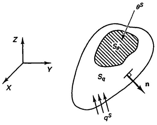# 7.2.1 Governing Heat Transfer Equations Consider a three-dimensional body in heat transfer conditions as shown in Fig. 7.1 and consider first steady-state conditions. For the heat transfer analysis we assume that the material obeys Fourier's law of heat conduction (see, for example, J. H. Lienhard [A]) 

text_image

Z Y X Sθ Sq θS n qS

Prescribed temperature $\theta^{S}$ on $S_{\theta}$ Prescribed heat flow input $q^{S}$ on $S_{q}$ Figure 7.1 Body subjected to heat transfer $$ q _ {x} = - k _ {x} \frac {\partial \theta}{\partial x}; \quad q _ {y} = - k _ {y} \frac {\partial \theta}{\partial y}; \quad q _ {z} = - k _ {z} \frac {\partial \theta}{\partial z} $$ where $q_{x}$ , $q_{y}$ , and $q_{z}$ are the heat flows conducted per unit area, $\theta$ is the temperature of the body, and $k_{x}$ , $k_{y}$ , $k_{z}$ are the thermal conductivities corresponding to the principal axes x, y, and z. Considering the heat flow equilibrium in the interior of the body, we thus obtain $$ \frac {\partial}{\partial x} \left(k _ {x} \frac {\partial \theta}{\partial x}\right) + \frac {\partial}{\partial y} \left(k _ {y} \frac {\partial \theta}{\partial y}\right) + \frac {\partial}{\partial z} \left(k _ {z} \frac {\partial \theta}{\partial z}\right) = - q ^ {B} \tag {7.1} $$ where $q^{B}$ is the rate of heat generated per unit volume. On the surfaces of the body the following conditions must be satisfied: $$ \theta | _ {s _ {\theta}} = \theta^ {s} \tag {7.2} $$ $$ k _ {n} \left. \frac {\partial \theta}{\partial n} \right| _ {s _ {q}} = q ^ {s} \tag {7.3} $$ where $\theta^{s}$ is the known surface temperature on $S_{\theta}$ , $k_{n}$ is the body thermal conductivity, n denotes the coordinate axis in the direction of the unit normal vector n (pointing outward) to the surface, $q^{s}$ is the prescribed heat flux input on the surface $S_{q}$ of the body, and $S_{\theta} \cup S_{q} = S$ , $S_{\theta} \cap S_{q} = 0$ . A number of important assumptions apply to the use of (7.1) to (7.3). A primary assumption is that the material particles of the body are at rest, and thus we consider the heat conduction conditions in solids and structures. If the heat transfer in a moving fluid is to be analyzed, it is necessary to include in (7.1) a term allowing for the convective heat transfer through the medium (see Section 7.4). Another assumption is that the heat transfer conditions can be analyzed decoupled from the stress conditions. This assumption is valid in many structural analyses, but may not be appropriate, for example, in the analysis of metal forming processes where the deformations may generate heat and change the temperature field. Such a change in turn may affect the material properties and result in further deformations. Another assumption is that there are no phase changes and latent heat effects (see Example 7.5 on how to incorporate such effects). However, we will assume in the following formulation that the material parameters are temperature-dependent.