Figure 7.4 shows for various Péclet numbers, $Pe = vL/\alpha$ , the exact solution to the problem in (7.94), given by $$ \frac {\theta - \theta_ {L}}{\theta_ {R} - \theta_ {L}} = \frac {\exp \left(\frac {\mathrm{Pe}}{L} x\right) - 1}{\exp (\mathrm{Pe}) - 1} \tag {7.96} $$ Hence, as Pe increases, the exact solution curve shows a strong boundary layer at $x = L$ . To demonstrate the inherent difficulty in the finite element solution, let us use two-node elements each of length h corresponding to a linearly varying temperature over each element. If we use the principle of virtual temperatures corresponding to $(7.73)$ (that is, we use the [standard] Galerkin method), we obtain for the finite element node i the governing equation $$ \left(- 1 - \frac {\mathrm{Pe} ^ {e}}{2}\right) \theta_ {i - 1} + 2 \theta_ {i} + \left(\frac {\mathrm{Pe} ^ {e}}{2} - 1\right) \theta_ {i + 1} = 0 \tag {7.97} $$ where the element Péclet number is $Pe^{e} = v h / \alpha$ . Hence $\theta_{i} = \frac{1 - \mathrm{Pe}^{e} / 2}{2}\theta_{i + 1} + \frac{1 + \mathrm{Pe}^{e} / 2}{2}\theta_{i - 1}$ (7.98) However, this equation already shows that for high values of $Pe^{e}$ , physically unrealistic results are obtained. 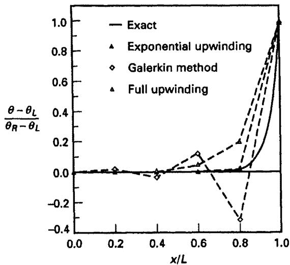For example, if $\theta_{i-1} = 0$ and $\theta_{i+1} = 100$ , we have $\theta_{i} = 50(1 - \mathrm{Pe}^{e}/2)$ , which gives a negative value if $Pe^{e} > 2!$ Figure 7.5 shows results obtained in the solution of the model problem in Fig. 7.4 with the two-node element discretization for the case Pe = 20 when using increasingly finer meshes. Actually, the analytical solution of (7.97) shows that for a reasonably accurate response prediction we need $Pe^{e}$ smaller than 2. This result is also reflected in Fig. 7.5 and means that a very fine mesh is required when Pe is large. In practical analyses, flows of very high Péclet and Reynolds numbers ( $Re \sim 10^{6}$ ) need be solved, and the finite element discretization scheme discussed in the previous section must be amended to be applicable to such problems. 

line

| x/L | Exact | Exponential upwinding | Galerkin method | Full upwinding | |-------|-------|------------------------|-----------------|----------------| | 0.0 | 0.0 | 0.0 | 0.0 | 0.0 | | 0.2 | 0.0 | 0.0 | 0.0 | 0.0 | | 0.4 | 0.0 | 0.0 | 0.0 | 0.0 | | 0.6 | 0.0 | 0.1 | 0.1 | 0.1 | | 0.8 | 0.0 | 0.2 | -0.3 | 0.2 | | 1.0 | 1.0 | 1.0 | 1.0 | 1.0 |

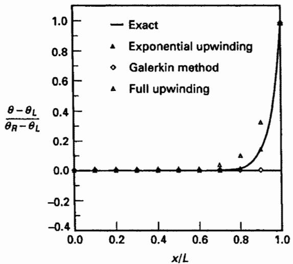
(a) Case of five elements, $Pe^{\theta}=4$ Figure 7.5 Solution of problem in Fig. 7.4 using two-node elements. Pe = 20. The exponential upwinding, Petrov-Galerkin, and Galerkin least squares methods give the exact values at the nodes. 

line

| x/L | Exact | Exponential upwinding | Galerkin method | Full upwinding | |-------|-------|------------------------|-----------------|----------------| | 0.0 | 0.0 | 0.0 | 0.0 | 0.0 | | 0.2 | 0.0 | 0.0 | 0.0 | 0.0 | | 0.4 | 0.0 | 0.0 | 0.0 | 0.0 | | 0.6 | 0.0 | 0.0 | 0.0 | 0.0 | | 0.8 | 0.0 | 0.0 | 0.0 | 0.0 | | 1.0 | 1.0 | 1.0 | 0.0 | 0.0 |

(b) Case of 10 elements, $Pe^{\theta}=2$ 

line

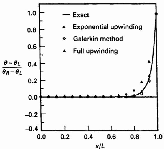
| x/L | Exact | Exponential upwinding | Galerkin method | Full upwinding | |-------|-------|------------------------|-----------------|----------------| | 0.0 | 0.0 | 0.0 | 0.0 | 0.0 | | 0.2 | 0.0 | 0.0 | 0.0 | 0.0 | | 0.4 | 0.0 | 0.0 | 0.0 | 0.0 | | 0.6 | 0.0 | 0.0 | 0.0 | 0.0 | | 0.8 | 0.0 | 0.0 | 0.0 | 0.0 | | 0.9 | 0.2 | 0.2 | 0.2 | 0.2 | | 0.95 | 0.4 | 0.4 | 0.4 | 0.4 | | 1.0 | 1.0 | 1.0 | 1.0 | 1.0 |

(c) Case of 15 elements, $Pe^{\theta}=4/3$ Figure 7.5 (continued) The shortcoming exposed above was recognized and overcome early by researchers using finite difference methods (see R. Courant, E. Isaacson, and M. Rees [A]). Namely, considering (7.97), we realize that this equation is also obtained when central differencing is used to solve (7.94) (see Section 3.3.5). Hence, the same solution inaccuracies are seen when the commonly employed central difference method is used to solve (7.94). The remedy designed to overcome the above difficulties is to use upwinding. In the finite difference upwind scheme, we use $$ \left. \frac {d \theta}{d x} \right| _ {i} \doteq \frac {\theta_ {i} - \theta_ {i - 1}}{h} \quad \text { if } v > 0 \tag {7.99} $$ $$ \frac {d \theta}{d x} | _ {i} \doteq \frac {\theta_ {i + 1} - \theta_ {i}}{h} \quad \text { if } v < 0 $$ In the following discussion we first assume $v > 0$ and then we generalize the results to consider any value of $v$ [see (7.115)]. If $v > 0$ , the finite difference approximation of (7.94) is $$ (- 1 - \mathrm{Pe} ^ {e}) \theta_ {i - 1} + (2 + \mathrm{Pe} ^ {e}) \theta_ {i} - \theta_ {i + 1} = 0 \tag {7.100} $$ Figure 7.5 shows the results obtained with this upwinding (denoted as “full upwinding”) for the problem being considered and shows that the oscillating solution behavior is no longer present. This solution improvement is explained by the nature of the (exact) analytical solution: if the flow is in the positive x-direction, the values of $\theta$ are influenced more by the upstream value $\theta_{L}$ than by the downstream value $\theta_{R}$ . Indeed, when Pe is large, the value of $\theta$ is close to the upstream value $\theta_{L}$ over much of the solution domain. The same observation holds when the flow is in the negative x-direction, but then $\theta_{R}$ is of course the upstream value. The intuitive implication of this observation is that in the finite difference discretization of $(7.94)$ , it should be appropriate to give more weight to the upstream value, and this is in essence accomplished in $(7.100)$ . Of course, it is desirable to further improve on the solution accuracy, and for the relatively simple (one-dimensional) equation $(7.94)$ , such improvement is obtained using different approaches. We briefly present below three such techniques that are actually closely related and result in excellent accuracy in one-dimensional analysis cases. However, the generalization of these methods to obtain small solution errors using relatively coarse discretizations in general two- and three-dimensional flow conditions is a difficult matter (see the end of this section). # Exponential Scheme The basic idea of the exponential scheme is to match the numerical solution to the analytical (exact) solution, which is known in the case considered here (see D. B. Spalding [A] and S. V. Patankar [A] for the development in control volume finite difference procedures). To introduce the scheme, let us rewrite (7.94) in the form $$ \frac {d f}{d x} = 0 \tag {7.101} $$ where the flux $f$ is given by the convective minus diffusive parts, $$ f = v \theta - \alpha \frac {d \theta}{d x} \tag {7.102} $$ The finite difference approximation of the relation in (7.101) for station i gives $$ f \left| _ {i + 1 / 2} - f \right| _ {i - 1 / 2} = 0 \tag {7.103} $$ This equation of course also corresponds to satisfying flux equilibrium for the control volume between the stations $i + \frac{1}{2}$ and $i - \frac{1}{2}$ . We now use the exact solution in (7.96) to express $f_{i+1/2}$ and $f_{i-1/2}$ in terms of the temperature values at the stations i - 1, i, $i + 1$ . Hence, using (7.96) for the interval i to $i + 1$ , we obtain $$ f _ {i + 1 / 2} = v \left[ \theta_ {i} + \frac {\theta_ {i} - \theta_ {i + 1}}{\exp (\mathrm{Pe} ^ {e}) - 1} \right] \tag {7.104} $$ Similarly, we obtain an expression for $f_{i-1/2}$ , and the relation (7.103) gives $$ (- 1 - c) \theta_ {i - 1} + (2 + c) \theta_ {i} - \theta_ {i + 1} = 0 \tag {7.105} $$ where $c = \exp\left(\mathrm{Pe}^{e}\right) - 1$ (7.106) We notice that for $Pe^{e} = 0$ the relation in (7.105) reduces to the use of the central difference method (and the Galerkin method) corresponding to the diffusive term only (because the convective term is zero) and that (7.105) has the form of (7.100) with c replacing $Pe^{e}$ . This scheme based on the analytical solution of the problem in Fig. 7.4 of course gives the exact solution even when only very few elements are used in the discretization (see Fig. 7.5). The scheme also yields very accurate solutions when the velocity v varies along the length of the domain considered and when source terms are included. A computational disadvantage is that the exponential functions need to be evaluated, and in practice it is sufficiently accurate and somewhat more effective to use a polynomial approximation instead of the (exact) analytical solution, which is referred to as the power law method. # Petrov-Galerkin Method Scheme with a Parameter The principle of virtual temperatures, as presented and used in Section 7.2, represents an application of the classical Galerkin method in which the same trial functions are used to express the weighting and the solution (see Section 3.3.3). However, in principle, different functions may be employed, and for certain types of problems such an approach can lead to increased solution accuracy. In the Petrov-Galerkin method, different functions are employed for the weighting than for the solution quantities. Let us assume that we are still using two-node elements to discretize the domain of the problem in Fig. 7.4. 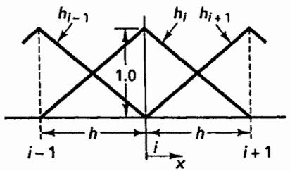Then the ith equation is $$ \int_ {- h} ^ {+ h} \tilde {h} _ {i} v \frac {d h _ {j}}{d x} \theta_ {j} d x + \int_ {- h} ^ {+ h} \frac {d \tilde {h} _ {i}}{d x} \alpha \frac {d h _ {j}}{d x} \theta_ {j} d x = 0 \quad j = i - 1, i, i + 1 \tag {7.107} $$ where $\tilde{h}_{i}$ denotes the weighting function and the $h_{j}$ are the usual functions of linear temperature distributions between nodes i - 1, i, and $i + 1$ (see Fig. 7.6). 

text_image

h_{i-1} \quad h_i \quad h_{i+1} \n 1.0 \n i-1 \quad h \quad i \quad h \quad i+1 \n x

Figure 7.6 Finite element functions used in (7.107) The basic idea is now to choose $\tilde{h}_{i}$ such as to obtain optimal accuracy. An efficient scheme to use is $$ \tilde {h} _ {i} = h _ {i} + \gamma \frac {h}{2} \frac {d h _ {i}}{d x} \quad \text { for } \nu > 0; \quad \tilde {h} _ {i} = h _ {i} - \gamma \frac {h}{2} \frac {d h _ {i}}{d x} \text { for } \nu < 0 \tag {7.108} $$ Using this weighting function in (7.107), we obtain for the case v > 0, $$ \left[ - 1 - \frac {\mathrm{Pe} ^ {e}}{2} (\gamma + 1) \right] \theta_ {i - 1} + (2 + \gamma \mathrm{Pe} ^ {e}) \theta_ {i} + \left[ - \frac {\mathrm{Pe} ^ {e}}{2} (\gamma - 1) - 1 \right] \theta_ {i + 1} = 0 \tag {7.109} $$ We note that with $\gamma = 0$ the standard Galerkin finite element equation in (7.97) is recovered, and when $\gamma = 1$ , the full upwind finite difference scheme in (7.100) is obtained. The variable $\gamma$ can be evaluated such that nodal exact values are obtained for all values of $\mathbf{Pe}^e$ (see I. Christie, D. F. Griffiths, A. R. Mitchell, and O. C. Zienkiewicz [A] and Exercise 7.19). $$ \gamma = \coth \left(\frac {\mathrm{Pe} ^ {e}}{2}\right) - \frac {2}{\mathrm{Pe} ^ {e}} \tag {7.110} $$ The case v < 0 is solved similarly. Of course, the results of our test problem in Fig. 7.5 using the Petrov-Galerkin method with the $\gamma$ value given above are the same as those using the exponential upwinding. # Flow-Condition-Based Interpolation Schemes Since the analytical solution to the one-dimensional problem is known, we can directly use it in constructing the finite element interpolation functions. This is the basic approach in the flow-condition-based interpolation (FCBI) schemes, see K.J. Bathe and H. Zhang [A]. In this approach the interpolation function for $\theta$ , the advection variable, is chosen based on the flow velocity conditions. Using again two-node elements, the governing ith equation is given by the Petrov-Galerkin formulation $$ \int_ {- h} ^ {+ h} h _ {i} v \frac {d \tilde {h} _ {j}}{d x} \theta_ {j} d x + \int_ {- h} ^ {+ h} \frac {d h _ {i}}{d x} \alpha \frac {d h _ {j}}{d x} \theta_ {j} d x = 0 \quad j = i - 1, i, i + 1 \tag {7.111} $$ where now the solution variable $\theta$ is interpolated in an element based on (7.96) using $\tilde{h}_j$ with $q = Pe^e / h$ $$ \tilde {h} _ {j} = 1 - \frac {\exp (q x) - 1}{\exp \left(\mathrm{Pe} ^ {e}\right) - 1} (\text { left node }) \quad \text { or } \quad \tilde {h} _ {j} = \frac {\exp (q x) - 1}{\exp \left(\mathrm{Pe} ^ {e}\right) - 1} (\text { right node }) \tag {7.112} $$ # Comparison of Methods Each of the above schemes gives of course the exact nodal point solutions in the one-dimensional solution of (7.94) and (7.95). The differences in the schemes arise when source terms are imposed and the schemes are used in multiple dimensions. An interesting observation and valuable interpretation is that all these methods are in essence equivalent to a Galerkin approximation with an additional diffusion term. Namely if we write the Galerkin solution of (7.94) with an additional diffusion term $\alpha\beta$ , we obtain $$ \int_ {- h} ^ {+ h} \left[ h _ {i} v \frac {d h _ {j}}{d x} \theta_ {j} + \frac {d h _ {i}}{d x} (1 + \beta) \alpha \frac {d h _ {j}}{d x} \theta_ {j} \right] d x = 0 \quad j = i - 1, i, i + 1 \tag {7.113} $$ where $\beta$ is a nondimensional constant, and we now consider v to be positive or negative. The solution of (7.113) is $$ - (1 + q) \theta_ {i - 1} + 2 \theta_ {i} - (1 - q) \theta_ {i + 1} = 0 \tag {7.114} $$ where $q = \frac{\mathrm{Pe}^e}{2}\frac{1}{1 + \beta}$ (7.115) The value of $\beta$ depends on which method is used, with $\beta = 0$ giving the standard Galerkin technique. Note that this observation does not suggest that we solve (7.94) with the diffusivity $(1 + \beta)\alpha$ . Instead, the observation shows that the above upwinding techniques give discretized equations obtained with the Galerkin method for the diffusivity $(1 + \beta)\alpha$ in order to obtain an accurate solution of (7.94). # Generalization of Techniques to Multi-dimensions With the excellent experiences of the schemes in one-dimensional solutions, the approaches seem attractive for the development of methods for general two- and three-dimensional flow conditions. In fluid flows, of course, the Reynolds number is used instead of the Péclet number. However, effective and accurate solution schemes for two- and three-dimensional complex flows have been difficult to reach. The difficulty is to have stability and obtain good accuracy in solutions. In finite difference control volume methods, the exponential and power law schemes (see Exercise 7.18) have been quite simply applied to the different coordinate directions using respective flow velocities, and generalizations have also been achieved; see, for example, W.J. Minkowycz, E.M. Sparrow, G.E. Schneider, and R.H. Pletcher [A]. For finite element analyses the Petrov-Galerkin scheme has been developed for general two- and three-dimensional solutions by applying, in essence, the one-dimensional scheme along the streamlines within each element, resulting in the streamline upwind Petrov-Galerkin (SuPG) method (see A.N. Brooks and T.J.R. Hughes [A] and C. Johnson, U. Nävert, and J. Pitkäranta [A]). The method can yield quite accurate and effective solutions when fine meshes are used but is not very stable, in particular when fluid-structure interaction solutions are sought, in which the boundary of the fluid domain changes. In such analyses, a flow-condition-based scheme can be more effective. Here the flow conditions establish interpolation functions for the advection terms along the element edges (see above) that are then interpolated over the element domain, see K.J. Bathe and H. Zhang [A] and H. Kohno and K.J. Bathe [A, B]. In addition, with the FCBI approach also a control volume-type scheme is used in the Galerkin formulation; for example, for the heat transfer equation $$ \int_ {V} w \left[ \nabla \cdot \left(\mathbf {v} \phi - \frac {1}{\mathrm{Pe}} \nabla \theta\right) \right] d V = 0 \tag {7.116} $$ where w is a constant weight function over the control volume V associated with the node. This approach enforces the momentum conditions strongly and directly on the nodes of the mesh (satisfying nodal and element properties like in solid mechanics, see Section 4.2.1) and provides for further stability (see K.J. Bathe and H. Zhang [A] and B. Banijamali and K.J. Bathe [A]). # 7.4.4 Fluid-Structure Interactions Based on the solution schemes of solids and structures and fluid flow problems, we can proceed to also briefly show how coupled fluid flow structural interactions (FSI) problems can be solved. Numerous publications have appeared on this subject, see for example S. Rugonyi and K. J. Bathe [A], K. J. Bathe and H. Zhang [B,C] and X. Wang [A] with the references therein, and various approaches can be followed for solutions. We shall only briefly focus here on a natural extension of the finite element procedures already presented in this book. Fundamentally, the discretizations of fluid flows and structures need to be coupled to satisfy the conditions of equilibrium (momentum transfer) and compatibility along the fluid-structure interfaces. Specific considerations arise because, in general, the fluid-structure boundaries will move and the meshes used for the structure and the fluid are quite different. For the structure a Lagrangian formulation is used in which the particles and boundaries are traced (the finite elements are attached to the material particles moving through space) and no special considerations arise for FSI solutions. However, for the fluid a pure Eulerian formulation is not adequate because then the boundaries must be stationary (the control volumes, and elements describing them, are fixed in space). Also, the fluid flow is typically solved using a much finer mesh than used for the structure. Since in general FSI solutions, the fluid domain changes as the structure deforms, an arbitrary Lagrangian-Eulerian (ALE) formulation can be used, see for example C. Nitikitpaiboon and K. J. Bathe [B]. Let $\mathfrak{v}$ be the fluid velocity and $\hat{\mathfrak{v}}$ be the velocity of a reference domain, then the time derivatives in the continuity, momentum and energy equations are obtained by considering an arbitray volume $V$ of the reference domain. For example, the continuity equation is $$ \frac {\partial}{\partial t} \left(\int_ {V} \rho d V\right) + \int_ {S} \rho (\mathbf {v} - \hat {\mathbf {v}}) \cdot \mathbf {n} d S = 0 \tag {7.117} $$ where S is the surface of V and n the outward unit normal to it. In practice, the velocity of the reference domain is the velocity of the finite element mesh used and for large motions of the boundary, this mesh needs to be moved incrementally, or even newly generated, throughout the finite element analysis of the FSI problem. Special algorithms based on the solution of Laplace equations and spring models have been established to calculate the new nodal point positions in the fluid mesh. Then the solution schemes discussed above for the structure and the fluid flow can directly be used. 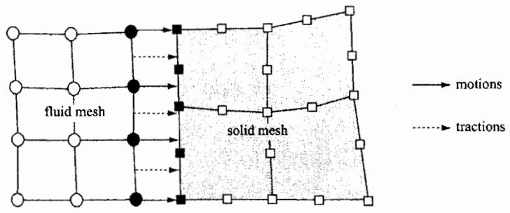However, throughout the solution, the fluid-structure interface conditions need to be satisfied. Referring to Fig. 7.7, the fluid mesh nodes are constrained to be on the solid boundary, they can slide along the solid elements (to preserve a good fluid mesh quality) but must stay on the boundary. As also implied in the figure, the tractions resulting from the fluid stresses in element m and represented as fluid nodal point forces $$ { } ^ { \prime } \mathbf { F } _ { f } ^ { ( m ) } = \int _ { V ^ { ( m ) } } \mathbf { B } ^ { T } { } ^ { t } \boldsymbol { \tau } ^ { ( m ) } d V ^ { ( m ) } \tag {7.118} $$ are applied to the structure, using the virtual work principle. In this way, the elementary patch tests are satisfied for the combined fluid-structure finite element assemblage, see K.J. Bathe and G.A. Ledezma [A]. For the solution of the FSI problems, the complete governing equations lead to $$ \left[ \begin{array}{l} ^ {t} \mathbf {F} _ {f} \\ ^ {t} \mathbf {F} _ {s - f} \\ ^ {t} \mathbf {F} _ {s} \end{array} \right] = \left[ \begin{array}{l} ^ {t} \mathbf {R} _ {f} \\ ^ {t} \mathbf {R} _ {s - f} \\ ^ {t} \mathbf {R} _ {s} \end{array} \right] \tag {7.119} $$ where the subscripts f and s denote the fluid and solid domains and s-f denotes the fluid-solid interface. 

flowchart

```mermaid graph TD A["●"] --> B["●"] B --> C["●"] C --> D["●"] D --> E["●"] E --> F["●"] F --> G["●"] G --> H["●"] H --> I["●"] I --> J["●"] J --> K["●"] K --> L["●"] L --> M["●"] M --> N["●"] N --> O["●"] O --> P["●"] P --> Q["●"] Q --> R["●"] R --> S["●"] S --> T["●"] T --> U["●"] U --> V["●"] V --> W["●"] W --> X["●"] X --> Y["●"] Y --> Z["●"] Z --> A["●"] style A fill:#fff,stroke:#000 style B fill:#fff,stroke:#000 style C fill:#fff,stroke:#000 style D fill:#fff,stroke:#000 style E fill:#fff,stroke:#000 style F fill:#fff,stroke:#000 style G fill:#fff,stroke:#000 style H fill:#fff,stroke:#000 style I fill:#fff,stroke:#000 style J fill:#fff,stroke:#000 style K fill:#fff,stroke:#000 style L fill:#fff,stroke:#000 style M fill:#fff,stroke:#000 style N fill:#fff,stroke:#000 style O fill:#fff,stroke:#000 style P fill:#fff,stroke:#000 style Q fill:#fff,stroke:#000 style R fill:#fff,stroke:#000 style S fill:#fff,stroke:#000 style T fill:#fff,stroke:#000 style U fill:#fff,stroke:#000 style V fill:#fff,stroke:#000 style W fill:#fff,stroke:#000 style X fill:#fff,stroke:#000 style Y fill:#fff,stroke:#000 style Z fill:#fff,stroke:#000 style AA fill:#fff,stroke:#000 style AB fill:#fff,stroke:#000 style AC fill:#fff,stroke:#000 style AD fill:#fff,stroke:#000 style AE fill:#fff,stroke:#000 style AF fill:#fff,stroke:#000 style AG fill:#fff,stroke:#000 style AH fill:#fff,stroke:#000 style AI fill:#fff,stroke:#000 style AJ fill:#fff,stroke:#000 style AK fill:#fff,stroke:#000 style AL fill:#fff,stroke:#000 style AM fill:#fff,stroke:#000 style AN fill:#fff,stroke:#000 style AO fill:#fff,stroke:#000 style AP fill:#fff,stroke:#000 style AQ fill:#fff,stroke:#000 style AR fill:#fff,stroke:#000 style AS fill:#fff,stroke:#000 style AT fill:#fff,stroke:#000 style AU fill:#fff,stroke:#000 style AV fill:#fff,stroke:#000 style AW fill:#fff,stroke:#000 style AX fill:#fff,stroke:#000 style AY fill:#fff,stroke:#000 style AZ fill:#fff,stroke:#000 style BA fill:#fff,stroke:#000 style BB fill:#fff,stroke:#000 style BC fill:#fff,stroke:#000 style BD fill:#fff,stroke:#000 style BE fill:#fff,stroke:#000 style BF fill:#fff,stroke:#000 style BG fill:#fff,stroke:#000 style BH fill:#fff,stroke:#000 style BI fill:#fff,stroke:#000 style BJ fill:#fff,stroke:#000 style BK fill:#fff,stroke:#000 style BL fill:#fff,stroke:#000 style BM fill:#fff,stroke:#000 style BN fill:#fff,stroke:#000 style BO fill:#fff,stroke:#000 style BP fill:#fff,stroke:#000 style BQ fill:#fff,stroke:#000 style CA fill:#fff,stroke:#000 style CB fill:#fff,stroke:#000 style CC fill:#fff,stroke:#000 style DD fill:#fff,stroke:#000 style DE fill:#fff,stroke:#000 style DF fill:#fff,stroke:#000 style DG fill:#fff,stroke:#000 style BEQ fill:#fff,stroke:#000 style BFQ fill:#fff,stroke:#000 style BGQ fill:#fff,stroke:#000 style BHQ fill:#fff,stroke:#000 style BIQ fill:#fff,stroke:#000 style BJQ fill:#fff,stroke:#000 style ACQ fill:#fff,stroke:#000 style ADQ fill:#fff,stroke:#000 style AEQ fill:#fff,stroke:#000 style AFQ fill:#fff,stroke:#000 style AGQ fill:#fff,stroke:#000 style AHQ fill:#fff,stroke:#000 style AIQ fill:#fff,stroke:#000 style AJQ fill:#fff,stroke:#000 style AKQ fill:#fff,stroke:#000 style ALQ fill:#fff,stroke:#000 style AMQ fill:#fff,stroke:#000 style ANQ fill:#fff,stroke:#000 style AOQ fill:#fff,stroke:#000 style APQ fill:#fff,stroke:#000 style AQQ fill:#fff,stroke:#000 style ARQ fill:#fff,stroke:#000 style ASQ fill:#fff,stroke:#000 style ATQ fill:#fff,stroke:#000 style AUQ fill:#fff,stroke:#000 style AVQ fill:#fff,stroke:#000 style AWQ fill:#fff,stroke:#000 style AXQ fill:#fff,stroke:#000 style AYQ fill:#fff,stroke:#000 style AZQ fill:#fff,stroke:#000 style BAQ fill:#fff,stroke:#000 style BBQ fill:#fff,stroke:#000 style BCQ fill:#fff,stroke:#000 style BDQ fill:#fff,stroke:#000 style BEQ fill:#fff,stroke:#000 style BFQ fill:#fff,stroke:#000 style BGQ fill:#fff,stroke:#000 style BHQ fill:#fff,stroke:#000 style BIQ fill:#fff,stroke:#000 style ADQ fill:#fff,stroke:#000 style AEQ fill:#fff,stroke:#000 style AFQ fill:#fff,stroke:#000 style AGQ fill:#fff,stroke:#000 style AHQ fill:#fff,stroke:#000 style AIQ fill:#fff,stroke:#000 style AJQ style AKQ style BBQ style BCQ style BDQ style BEQ style BFQ style BGQ style BHQ style BIQ style ADQ style AFQ style AGQ style AHQ style AIQ style AJQ style AKQ style BFQ style BGQ style BHQ style BIQ style ADQ style AEQ style AFQ style AGQ style AHQ style AIQ style AJQ style AKQ style BFQ style BGQ style BHQ style BIQ style ADQ style AFQ style AGQ style AHQ style AIQ style AJQ style AKQ style BFQ style BGQ style BHQ style BIQ style ADQ style AFQ style AGQ style AHQ style AIQ style AJQ style AKQ style BFQ style BGQ style BIQ style ADQ style AEQ style AFQ style AGQ style AHQ style AIQ style AJQ style AKQ style BFQ style BGQ style BHQ style BIQ style ADQ style AFQ style AGQ style AHQ style AIQ style AJQ styleAKQ style BFQ style BGQ style BHQ style BIQ style ADQ style AFQ style AGQ style AHQ style AIQ style AJQ style AKQ style BFQ style BGQ style BHQ style BIQ style ADQ style AFQ style AGQ style AHQ style AJQ style AKQ style BFQ style BGQ style BHQ style BIQ style ADQ style AFQ style AGQ style AHQ style AIQ style AJQ style AKQ style BFQ style BGQ style BHQ style BIQ style ADQ style AFQ style ACQ style ADQ fill:#fff,stroke:#000 style AEQ fill:#fff,stroke:#000 style AFQ fill:#fff,stroke:#000 style AGQ fill:#fff,stroke:#000 style AHQ fill:#fff,stroke:#000 style AIQ fill:#fff,stroke:#000 style AJQ fill:#fff,stroke:#000 ``` ```

Figure 7.7 Schematic of conditions at FSI interface Here the interface conditions are contained in (7.119). The unknowns are the nodal displacements (and if applicable rotations) in the solid or structure, the nodal fluid velocities, the fluid element or nodal pressures, the nodal temperatures, and the nodal positions of the fluid mesh (separately solved for). The equations (7.119) are solved using an iterative scheme, where a full Newton-Raphson direct sparse solver solution may require a large coefficient matrix and significant memory and solution time. Irrespective of which iterative scheme is used, of course, the fully coupled solution is obtained once convergence has been reached to satisfy (7.119), see K.J. Bathe, H. Zhang, and S. Ji [A] and K. J. Bathe and H. Zhang [B]. The above scheme is very general, since all mechanical conditions are satisfied. In some analyses, simplifying assumptions can be used. For example, if the structure is very stiff, it may be assumed that the fluid domain does not change. Then the complete fluid analysis may first be carried out and thereafter the fluid actions are applied to the structure (referred to as one-way coupling). For lightly coupled systems, it may be sufficient to use a staggered solution procedure, in which the structure and fluid domains are solved separately and the interactions are lagging a solution step behind. # 7.4.5 Exercises 7.15. Starting with the basic equations (7.57) to (7.60), derive (7.65) and then also derive (7.67) and (7.68). 7.16. Show in detail that the matrix expressions for the two-dimensional planar flow conditions given in (7.77) to (7.89) are correct. 7.17. Consider that the matrix equations in (7.77) are to be solved for the steady-state case using a full Newton-Raphson iteration. Develop the coefficient matrix and give all details of the evaluations to be performed. 7.18. Derive the expressions for upwinding given in (7.105) and (7.106). 7.19. Derive the expressions for upwinding given in (7.109) and (7.110). 7.20. Establish the equation for node i in (7.111) for the FCBI scheme. 7.21. Show analytically that the equations (7.105), (7.109) and (7.111) give identical solutions. 7.22. Show that the solution of (7.113) is given by (7.114) and (7.115), and give $\beta$ for the scheme of (7.109). 7.23. Prove that the ALE equation (7.117) is correct and derive the momentum and energy equations. 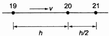7.24. Derive the governing finite element equation for the solution of (7.94) for node 20 of the assemblage of the two-node elements shown. (a) Use the FCBI scheme. (b) Use full upwinding. 

text_image

19 → v 20 21 h h/2

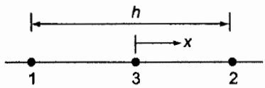
Constant velocity v Cross-sectional area = 1.0 7.25. Consider the three-node one-dimensional element shown for the solution of (7.94). Show that the bubble function $\tilde{h}_3$ introduces, in essence, upwinding in the element. [Hint: Apply the Galerkin procedure to the element and evaluate the value of $\beta$ when comparing the equations you have established with (7.113).] See F. Brezzi and A. Russo [A]. 

text_image

h x 1 3 2

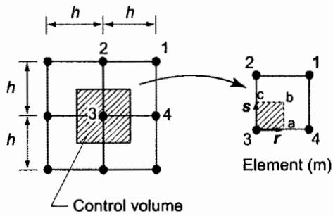
$$ h _ {1} = \frac {1}{2} (1 - \frac {2 x}{h}); h _ {2} = \frac {1}{2} (1 + \frac {2 x}{h}) $$ $$ \tilde {h} _ {3} = 1 - \left(\frac {2 x}{h}\right) ^ {2} $$ 7.26. Consider the two-dimensional element shown. Develop a flow-condition based scheme for this element for heat transfer analysis based on (7.116). Here use the functions (7.112) along opposing element edges and a linear variation across. 

text_image

h h 2 1 h 3 4 Control volume 2 1 s c b 3 r a 4 Element (m)

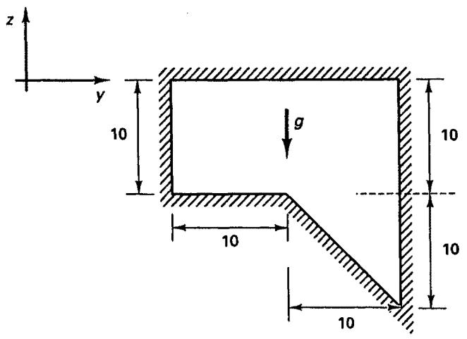
7.27. Consider the water-filled cavity acted upon by gravity as shown. Use a computer program to calculate (with a very coarse mesh) the velocities (to be calculated as zero, of course) and the pressure distribution in the water. Prescribe that the velocities are zero on the boundary (but calculate “unknown” velocities in the domain). $$ g = 1 0 $$ $$ \rho = 1. 0 $$ $$ p = 0 \text { at } z = 0 $$ 

text_image

z y 10 g 10 10 10 10

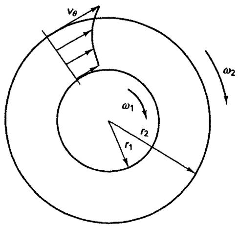
7.28. Use a computer program to analyze the fully developed flow between two concentric cylinders rotating at speeds $\omega_{1}$ and $\omega_{2}$ as shown. Verify that an accurate solution has been obtained. 

text_image

vθ ω1 r2 r1 ω2

$$ r _ {1} = 1; r _ {2} = 2; $$ $$ \omega_ {1} = 1; \omega_ {2} = 2; $$ $$ \rho = 1; \mu = 1; $$