```csv
I=I + 1 SSP00562
IF (I.LE.NROOT) GO TO 270 SSP00563
BUPC(L)=BUP(I-1) SSP00564
290 LM=L SSP00565
IF (NROOT.EQ.NC) GO TO 300 SSP00566
295 IF (BUP(I-1).LE.BLO(I)) GO TO 300 SSP00567
IF (RTOLV(I).GT.RTOL) GO TO 300 SSP00568
BUPC(L)=BUP(I) SSP00569
NEIV(L)=NEIV(L) + 1 SSP00570
NROOT=NROOT + 1 SSP00571
IF (NROOT.EQ.NC) GO TO 300 SSP00572
I=I + 1 SSP00573
GO TO 295 SSP00574
C SSP00575
C FIND SHIFT SSP00576
C SSP00577
300 WRITE (IOUT,1020) SSP00578
WRITE (IOUT,1005) (BUPC(I),I=1,LM) SSP00579
WRITE (IOUT,1030) SSP00580
WRITE (IOUT,1006) (NEIV(I),I=1,LM) SSP00581
LL=LM - 1 SSP00582
IF (LM.EQ.1) GO TO 310 SSP00583
330 DO 320 I=1,LL SSP00584
320 NEIV(L)=NEIV(L) + NEIV(I) SSP00585
L=L - 1 SSP00586
LL=LL - 1 SSP00587
IF (L.NE.1) GO TO 330 SSP00588
310 WRITE (IOUT,1040) SSP00589
WRITE (IOUT,1006) (NEIV(I),I=1,LM) SSP00590
L=0 SSP00591
DO 340 I=1,LM SSP00592
L=L + 1 SSP00593
IF (NEIV(I).GE.NROOT) GO TO 350 SSP00594
340 CONTINUE SSP00595
350 SHIFT=BUPC(L) SSP00596
NEI=NEIV(L) SSP00597
GO TO 900 SSP00598
C SSP00599
800 STOP SSP00600
900 RETURN SSP00601
C SSP00602
1005 FORMAT ( ' ',6E22.14) SSP00603
1006 FORMAT ( ' ',6I22) SSP00604
1010 FORMAT ( ' *** ERROR *** SOLUTION STOP IN *SCHECK* ',/, SSP00605
1 ' NO EIGENVALUES FOUND ',/ ) SSP00606
1020 FORMAT (///,' UPPER BOUNDS ON EIGENVALUE CLUSTERS') SSP00607
1030 FORMAT (///,' NO. OF EIGENVALUES IN EACH CLUSTER') SSP00608
1040 FORMAT ( ' NO. OF EIGENVALUES LESS THAN UPPER BOUNDS') SSP00609
END SSP00610
SUBROUTINE JACOBI (A,B,X,EIGV,D,N,NWA,RTOL,NSMAX,IFPR,IOUT) SSP00611
C SSP00612
C . SSP00613
C . P R O G R A M . SSP00614
C . TO SOLVE THE GENERALIZED EIGENPROBLEM USING THE . SSP00615
C . GENERALIZED JACOBI ITERATION . SSP00616
C . IMPLICIT DOUBLE PRECISION (A-H,O-Z) SSP00617
DIMENSION A(NWA),B(NWA),X(N,N),EIGV(N),D(N) SSP00618
C SSP00619
C INITIALIZE EIGENVALUE AND EIGENVECTOR MATRICES SSP00620
C SSP00621
N1=N + 1 SSP00622
II=1 SSP00623
DO 10 I=1,N SSP00624
IF (A(II).GT.0. .AND. B(II).GT.0.) GO TO 4 SSP00625
WRITE (IOUT,2020) II,A(II),B(II) SSP00626
GO TO 800 SSP00627
4 D(I)=A(II)/B(II) SSP00628
EIGV(I)=D(I) SSP00629
10 II=II + N1 - I SSP00630
C SSP00631
```
```csv
DO 30 I=1,N
DO 20 J=1,N
20 X(I,J)=0.
30 X(I,I)=1.
IF (N.EQ.1) GO TO 900
INITIALIZE SWEEP COUNTER AND BEGIN ITERATION
NSWEEP=0
NR=N - 1
40 NSWEEP=NSWEEP + 1
IF (IFPR.EQ.1) WRITE (IOUT,2000) NSWEEP
CHECK IF PRESENT OFF-DIAGONAL ELEMENT IS LARGE ENOUGH TO REQUIRE ZEROING
EPS=(.01)**(NSWEEP*2)
DO 210 J=1,NR
JP1=J + 1
JM1=J - 1
LJK=JM1*N - JM1*J/2
JJ=LJK + J
DO 210 K=JP1,N
KP1=K + 1
KM1=K - 1
JK=LJK + K
KK=KM1*N - KM1*K/2 + K
EPTOLA=(A(JK)/A(JJ))*(A(JK)/A(KK))
EPTOLB=(B(JK)/B(JJ))*(B(JK)/B(KK))
IF (EPTOLA.LT.EPS .AND. EPTOLB.LT.EPS) GO TO 210
IF ZEROING IS REQUIRED, CALCULATE THE ROTATION MATRIX ELEMENTS CA AND CG
AKK=A(KK)*B(JK) - B(KK)*A(JK)
AJJ=A(JJ)*B(JK) - B(JJ)*A(JK)
AB=A(JJ)*B(KK) - A(KK)*B(JJ)
SCALE=A(KK)*B(KK)
ABCH=AB/SCALE
AKKCH=AKK/SCALE
AJJCH=AJJ/SCALE
CHECK=(ABCH*ABCH+4.0*AKKCH*AJJCH)/4.0
IF (CHECK) 50,60,60
50 WRITE (IOUT,2020) JJ,A(JJ),B(JJ)
GO TO 800
60 SQCH=SCALE*SQRT(CHECK)
D1=AB/2. + SQCH
D2=AB/2. - SQCH
DEN=D1
IF (ABS(D2).GT.ABS(D1)) DEN=D2
IF (DEN) 80,70,80
70 CA=0.
CG=-A(JK)/A(KK)
GO TO 90
80 CA=AKK/DEN
CG=-AJJ/DEN
PERFORM THE GENERALIZED ROTATION TO ZERO THE PRESENT OFF-DIAGONAL ELEMENT
90 IF (N-2) 100,190,100
10 IF (JM1-1) 130,110,110
10 DO 120 I=1,JM1
IM1=I - 1
IJ=IM1*N - IM1*I/2 + J
IK=IM1*N - IM1*I/2 + K
AJ=A(IJ)
BJ=B(IJ)
AK=A(IK)
BK=B(IK)
SSP00632
SSP00633
SSP00634
SSP00635
SSP00636
SSP00637
SSP00638
SSP00639
SSP00640
SSP00641
SSP00642
SSP00643
SSP00644
SSP00645
SSP00646
SSP00647
SSP00648
SSP00649
SSP00650
SSP00651
SSP00652
SSP00653
SSP00654
SSP00655
SSP00656
SSP00657
SSP00658
SSP00659
SSP00660
SSP00661
SSP00662
SSP00663
SSP00664
SSP00665
SSP00666
SSP00667
SSP00668
SSP00669
SSP00670
SSP00671
SSP00672
SSP00673
SSP00674
SSP00675
SSP00676
SSP00677
SSP00678
SSP00679
SSP00680
SSP00681
SSP00682
SSP00683
SSP00684
SSP00685
SSP00686
SSP00687
SSP00688
SSP00689
SSP00690
SSP00691
SSP00692
SSP00693
SSP00694
SSP00695
SSP00696
SSP00697
SSP00698
SSP00699
SSP00700
SSP00701
```
```csv
A(IJ)=AJ + CG*AK
B(IJ)=BJ + CG*BK
A(IK)=AK + CA*AJ
120 B(IK)=BK + CA*BJ
130 IF (KP1-N) 140,140,160
140 LJI=JM1*N - JM1*J/2
LKI=KM1*N - KM1*K/2
DO 150 I=KP1,N
JI=LJI + I
KI=LKI + I
AJ=A(JI)
BJ=B(JI)
AK=A(KI)
BK=B(KI)
A(JI)=AJ + CG*AK
B(JI)=BJ + CG*BK
A(KI)=AK + CA*AJ
150 B(KI)=BK + CA*BJ
160 IF (JP1-KM1) 170,170,190
170 LJI=JM1*N - JM1*J/2
DO 180 I=JP1,KM1
JI=LJI + I
IM1=I - 1
IK=IM1*N - IM1*I/2 + K
AJ=A(JI)
BJ=B(JI)
AK=A(IK)
BK=B(IK)
A(JI)=AJ + CG*AK
B(JI)=BJ + CG*BK
A(IK)=AK + CA*AJ
180 B(IK)=BK + CA*BJ
190 AK=A(KK)
BK=B(KK)
A(KK)=AK + 2.*CA*A(JK) + CA*CA*A(JJ)
B(KK)=BK + 2.*CA*B(JK) + CA*CA*B(JJ)
A(JJ)=A(JJ) + 2.*CG*A(JK) + CG*CG*AK
B(JJ)=B(JJ) + 2.*CG*B(JK) + CG*CG*BK
A(JK)=0.
B(JK)=0.
C
C
C
C
C
C
C
C
C
C
C
C
C
C
C
C
C
C
C
C
C
C
C
C
C
C
C
C
C
C
C
C
C
C
C
C
C
C
C
C
C
C
C
C
C
C
C
C
C
C
C
```
```csv
C
C CHECK ALL OFF-DIAGONAL ELEMENTS TO SEE IF ANOTHER SWEEP IS
C REQUIRED
C
EPS=RTOL**2
DO 250 J=1,NR
JM1=J - 1
JP1=J + 1
LJK=JM1*N - JM1*J/2
JJ=LJK + J
DO 250 K=JP1,N
KM1=K - 1
JK=LJK + K
KK=KM1*N - KM1*K/2 + K
EPSA=(A(JK)/A(JJ))*(A(JK)/A(KK))
EPSB=(B(JK)/B(JJ))*(B(JK)/B(KK))
IF (EPSA.LT.EPS .AND. EPSB.LT.EPS) GO TO 250
GO TO 280
250 CONTINUE
C
C SCALE EIGENVECTORS
C
255 II=1
DO 275 I=1,N
BB=SQRT(B(II))
DO 270 K=1,N
270 X(K,I)=X(K,I)/BB
275 II=II + N1 - I
GO TO 900
C
C UPDATE D MATRIX AND START NEW SWEEP, IF ALLOWED
C
280 DO 290 I=1,N
290 D(I)=EIGV(I)
IF (NSWEEP.LT.NSMAX) GO TO 40
GO TO 255
C
800 STOP
900 RETURN
C
2000 FORMAT (//,' SWEEP NUMBER IN *JACOB1* = ',I8)
2010 FORMAT ( ' ',6E20.12)
2020 FORMAT ( ' *** ERROR *** SOLUTION STOP',/,
1 ' MATRICES NOT POSITIVE DEFINITE',/,
2 ' II = ',I8,' A(II) = ',E20.12,' B(II) = ',E20.12)
2030 FORMAT (//,' CURRENT EIGENVALUES IN *JACOB1* ARE',/)
END
SSP00772
SSP00773
SSP00774
SSP00775
SSP00776
SSP00777
SSP00778
SSP00779
SSP00780
SSP00781
SSP00782
SSP00783
SSP00784
SSP00785
SSP00786
SSP00787
SSP00788
SSP00789
SSP00790
SSP00791
SSP00792
SSP00793
SSP00794
SSP00795
SSP00796
SSP00797
SSP00798
SSP00799
SSP00800
SSP00801
SSP00802
SSP00803
SSP00804
SSP00805
SSP00806
SSP00807
SSP00808
SSP00809
SSP00810
SSP00811
SSP00812
SSP00813
SSP00814
SSP00815
SSP00816
SSP00817
SSP00818
```
The subspace iteration program presented here is for the solution of the smallest eigenvalues and corresponding eigenvectors, where p is assumed to be small (say $p \leq 20$ ). Considering the solution of problems for a larger number of eigenpairs, the formula $q = \max\{2p, p + 8\}$ should be used, see K.J. Bathe [J].
Of course, in practice procedures for accelerating the basic subspace iteration solution given in subroutine SSPACE are very desirable, in particular, when a larger number of eigenpairs is to be calculated. Various acceleration procedures for the basic subspace iteration method have indeed been proposed, see for example K. J. Bathe and S. Ramaswamy [A], F.A. Dul and K. Arczewski [A], Q. C. Zhao, P. Chen, W. B. Peng, Y. C. Gong, and M. W. Yuan [A] and K. J. Bathe and J. Dong [A].
# 11.6.6 Exercises
11.18. Show explicitly that the iteration vectors $\mathbf{X}_{k + 1}$ in the subspace iteration are $\mathbf{K}$ - and $\mathbf{M}$ -orthogonal.
11.19. Use two iteration vectors in the subspace iteration method to solve for the two smallest eigenvalues and corresponding eigenvectors of the problem considered in Exercise 11.1.
11.20. Show that in the subspace iteration the use of (10.107) results after $(k-1)$ iterations into
$$
\left[ 1 - \frac {\left(\lambda_ {i} ^ {(k)}\right) ^ {2}}{\left(\mathbf {q} _ {i} ^ {(k)}\right) ^ {T} \mathbf {q} _ {i} ^ {(k)}} \right] ^ {1 / 2} \leq t o l
$$
where $\lambda_{i}^{(k)}$ is the calculated eigenvalue approximation and $\mathbf{q}_{i}^{(k)}$ is the corresponding eigenvector in $\mathbf{Q}_{k}$ .
11.21. The number of numerical operations used in program SSPACE can be decreased at the expense of using more memory. Then no additional iteration is performed after convergence. Reprogram SSPACE to achieve this decrease in numerical operations used.
11.22. Develop a program such as SSPACE using the programming language C (instead of Fortran), and compare the efficiencies of the two implementations.
# Implementation of the Finite Element Method
# 12.1 INTRODUCTION
In this book we have presented formulations, general theories, and numerical methods of finite element analysis. The objective in this final chapter is to discuss some important computational aspects pertaining to the implementation of finite element procedures. Although the implementation of displacement-based finite element analysis is discussed, it should be noted that most of the concepts presented can also be employed in finite element analysis using mixed formulations. Note, in particular, that the mixed interpolations of the u/p formulation for two- and three-dimensional continuum elements (see Sections 4.4.3, 5.3.5, and 6.4) and the mixed interpolations for beam, plate, and shell elements (see Sections 5.4 and 6.5) have only nodal displacements and rotations as final element degrees of freedom, and hence the process of element assemblage and solution of equations is as in the pure displacement-based formulation.
The main advantage that the finite element method has over other analysis techniques is its large generality. Normally, as was pointed out, it seems possible, by using many elements, to virtually approximate any continuum with complex boundary and loading conditions to such a degree that an accurate analysis can be carried out. In practice, however, obvious engineering limitations arise, a most important one being the cost of the analysis. This cost consists of the purchase and/or leasing of hardware and software, the analyst's effort and time required to prepare the analysis input data, the computer program execution time, and the analyst's time to interpret the results. Of course, as discussed in Section 1.2, a number of program runs may be required. Also, the limitations of the computer and the program employed may prevent the use of a sufficiently fine discretization to obtain accurate results. Hence, it is clearly desirable to use an efficient finite element program.
The effectiveness of a program depends essentially on the following factors. First, the use of efficient finite elements is important.
Second, efficient programming methods and sophisticated use of the available computer hardware and software are important. Although this aspect of program development
is computer-dependent, using standard FORTRAN 77 or C and high- and low-speed storage in a system-independent manner, very effective computer programs can be developed. If such a program is to be permanently installed on a specific computer, its efficiency may normally be increased with relatively little effort by making use of the specific hardware and software options available. In the following, we therefore discuss the design of finite element programs in which largely computer-independent procedures are used.
The third very important aspect of the development of a finite element program is the use of appropriate numerical techniques. As an example, if inappropriate techniques for the solution of the frequencies of a system in a dynamic analysis are employed, the cost may be many times greater than with effective techniques, and, even worse, a solution may not be possible at all if an unstable algorithm is employed. In order to implement the finite element method in practice, we need to use the digital computer. However, even with a relatively large-capacity computer available, the feasibility of a problem solution and the effectiveness of an analysis depend directly on the numerical procedures employed.
Assume that an actual structure has been idealized as an assemblage of finite elements. The stress analysis process can be understood to consist of essentially three phases:
1. Calculation of system matrices K, M, C, and R, whichever are applicable.
2. Solution of equilibrium equations.
3. Evaluation of element stresses.
In the analysis of a heat transfer, field, or fluid mechanics problem, the steps are identical, but the pertinent matrices and solution quantities need to be used.
The objective in this chapter is to describe a program implementation of the first and third phases and to present a small computer program that has all the important features of a general code. Although the total solution may be subdivided into the above three phases, it should be realized that the specific implementation of one phase can have a pronounced effect on the efficiency of another phase, and, indeed, in some programs the first two phases are carried out simultaneously (e.g., when using the frontal solution method; see Section 8.2.4).
As might be imagined, there is no unique optimum program organization for the evaluation of the system matrices; however, although program designs may appear to be quite different, in effect, some basic steps are followed. For this reason, it is most instructive to discuss in detail all the important features of one implementation that is based on classical methods. First we discuss the algorithms used, and then we present a small example program. This implementation is for a single processor machine but can be adapted for use of multiple processors and parallel computing.
# 12.2 COMPUTER PROGRAM ORGANIZATION FOR CALCULATION OF SYSTEM MATRICES
The final results of this phase are the required structure matrices for the solution of the system equilibrium equations. In a static analysis the computer program needs to calculate the structure stiffness matrix and the load vectors. In a dynamic analysis, the program must also establish the system mass and damping matrices. In the implementation to be described here, the calculation of the structure matrices is performed as follows.
1. The nodal point and element information are read and/or generated.
2. The element stiffness matrices, mass and damping matrices, and equivalent nodal loads are calculated.
3. The structure matrices K, M, C, and R, whichever are applicable, are assembled.
# 12.2.1 Nodal Point and Element Information Read-in
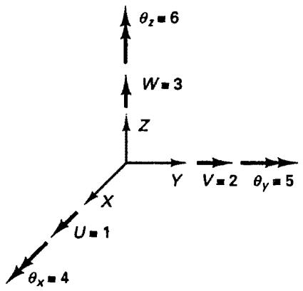
Consider first the data that correspond to the nodal points. Assume that the program is set up to allow a maximum of six degrees of freedom at each node, three translational and three rotational degrees of freedom, as shown in Fig. 12.1. Corresponding to each nodal point, it must then be identified which of these degrees of freedom shall actually be used in the analysis, i.e., which of the six possible nodal degrees of freedom correspond to degrees of freedom of the finite element assemblage. This is achieved by defining an identification array, the array ID, of dimension 6 times NUMNP, where NUMNP is equal to the number of nodal points in the system. Element $(i, j)$ in the ID array corresponds to the ith degree of freedom at the nodal point j. If ID(I, J) = 0, the corresponding degree of freedom is defined in the global system, and if ID(I, J) = 1, the degree of freedom is not defined. It should be noted that using the same procedure, an ID array for more (or less) than six degrees of freedom per nodal point could be established, and, indeed, the number of degrees of freedom per nodal point could be a variable. Consider the following simple example.
text_image
θz = 6
W = 3
Z
Y
V = 2 θy = 5
X
U = 1
θx = 4
Figure 12.1 Possible degrees of freedom at a nodal point
EXAMPLE 12.1: Establish the ID array for the plane stress element idealization of the cantilever in Fig. E12.1 in order to define the active and nonactive degrees of freedom.
The active degrees of freedom are defined by $ID(I, J) = 0$ , and the nonactive degrees of freedom are defined by $ID(I, J) = 1$ . Since the cantilever is in the X, Y plane and plane stress elements are used in the idealization, only X and Y translational degrees of freedom are active. By inspection, the ID array is given by
$$
\mathbf {I D} = \left[ \begin{array}{c c c c c c c c c} 1 & 1 & 1 & 0 & 0 & 0 & 0 & 0 & 0 \\ 1 & 1 & 1 & 0 & 0 & 0 & 0 & 0 & 0 \\ 1 & 1 & 1 & 1 & 1 & 1 & 1 & 1 & 1 \\ 1 & 1 & 1 & 1 & 1 & 1 & 1 & 1 & 1 \\ 1 & 1 & 1 & 1 & 1 & 1 & 1 & 1 & 1 \\ 1 & 1 & 1 & 1 & 1 & 1 & 1 & 1 & 1 \end{array} \right]
$$
text_image
Temperature at top face = 100°C
60 cm
60 cm
12
11
40 cm
40 cm
40 cm
Node
number
Temperature at
bottom face = 70°C
6
6
5
9
Element
number
E = 10⁶ N/cm²
v = 0.15
4
E = 2 × 10⁶ N/cm²
v = 0.20
10
2
5
3
8
9
1
3
1
2
E = 10⁶ N/cm²
v = 0.15
2
E = 2 × 10⁶ N/cm²
v = 0.20
8
1
4
7
7
Degree of
freedom
number
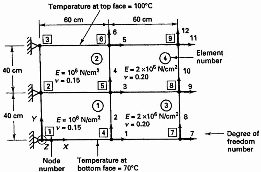
Figure E12.1 Finite element cantilever idealization
Once all active degrees of freedom have been defined by zeros in the ID array, the equation numbers corresponding to these degrees of freedom are assigned. The procedure is to simply scan column after column through the ID array and replace each zero by an equation number, which increases successively from 1 to the total number of equations. At the same time, the entries corresponding to the nonactive degrees of freedom are set to zero.
EXAMPLE 12.2: Modify the ID array obtained in Example 12.1 for the analysis of the cantilever plate in Fig. E12.1 to obtain the ID array that defines the equation numbers corresponding to the active degrees of freedom.
As explained above, we simply replace the zeros, column by column, in succession by equation numbers to obtain
$$
\mathbf {I D} = \left[ \begin{array}{c c c c c c c c c} 0 & 0 & 0 & 1 & 3 & 5 & 7 & 9 & 1 1 \\ 0 & 0 & 0 & 2 & 4 & 6 & 8 & 1 0 & 1 2 \\ 0 & 0 & 0 & 0 & 0 & 0 & 0 & 0 & 0 \\ 0 & 0 & 0 & 0 & 0 & 0 & 0 & 0 & 0 \\ 0 & 0 & 0 & 0 & 0 & 0 & 0 & 0 & 0 \\ 0 & 0 & 0 & 0 & 0 & 0 & 0 & 0 & 0 \end{array} \right]
$$
Apart from the definition of all active degrees of freedom, we also need to read the X, Y, Z global coordinates and, if required, the temperature corresponding to each nodal point. For the cantilever beam in Fig. E12.1, the X, Y, Z coordinate arrays and nodal point temperature array T would be as follows:
$$
\begin{array}{l} \mathrm{X} = \left[ \begin{array}{l l l l l l l l l l} 0. 0 & 0. 0 & 0. 0 & 6 0. 0 & 6 0. 0 & 6 0. 0 & 1 2 0. 0 & 1 2 0. 0 & 1 2 0. 0 \end{array} \right] \\ \begin{array}{l} \mathrm{Y} = [ 0. 0 \quad 4 0. 0 \quad 8 0. 0 \quad 0. 0 \quad 4 0. 0 \quad 8 0. 0 \quad 0. 0 \quad 4 0. 0 \quad 8 0. 0 ] \\ \text {T} = [ 0. 0 \quad 4 0. 0 \quad 8 0. 0 \quad 0. 0 \quad 4 0. 0 \quad 8 0. 0 \quad 0. 0 \quad 4 0. 0 \quad 8 0. 0 ] \end{array} \tag {12.1} \\ Z = \left[ \begin{array}{l l l l l l l l l l} 0. 0 & 0. 0 & 0. 0 & 0. 0 & 0. 0 & 0. 0 & 0. 0 & 0. 0 & 0. 0 & 0. 0 \end{array} \right] \\ \mathbf {T} = \left[ \begin{array}{l l l l l l l l l} 7 0. 0 & 8 5. 0 & 1 0 0. 0 & 7 0. 0 & 8 5. 0 & 1 0 0. 0 & 7 0. 0 & 8 5. 0 & 1 0 0. 0 \end{array} \right] \\ \end{array}
$$
At this stage, with all the nodal point data known, the program may read and generate the element information. It is expedient to consider each element type in turn. For example,
in the analysis of a container structure, all beam elements, all plane stress elements, and all shell elements are read and generated together. This is efficient because specific information must be provided for each element of a certain type, which, because of its repetitive nature, can be generated to some degree if all elements of the same type are specified together. Furthermore, the element routine for an element type that reads the element data and calculates the element matrices needs to be called only once.
The required data corresponding to an element depend on the specific element type. In general, the information required for each element is the element node numbers that correspond to the nodal point numbers of the complete element assemblage, the element material properties, and the surface and body forces applied to the element. Since the element material properties and the element loading are the same for many elements, it is efficient to define material property sets and load sets pertaining to an element type. These sets are specified at the beginning of each group of element data. Therefore, any one of the material property sets and element load sets can be assigned to an element at the same time the element node numbers are read.
EXAMPLE 12.3: Consider the analysis of the cantilever plate shown in Fig. E12.1 and the local element node numbering defined in Fig. 5.4. For each element give the node numbers that correspond to the nodal point numbers of the complete element assemblage. Also indicate the use of material property sets.
In this analysis we define two material property sets: material property set 1 for $E = 10^{6}$ N/cm $^{2}$ and $\nu = 0.15$ , and material property set 2 for $E = 2 \times 10^{6}$ N/cm $^{2}$ and $\nu = 0.20$ . We then have the following node numbers and material property sets for each element:
Element 1: node numbers: 5, 2, 1, 4; material property set: 1
Element 2: node numbers: 6, 3, 2, 5; material property set: 1
Element 3: node numbers: 8, 5, 4, 7; material property set: 2
Element 4: node numbers: 9, 6, 5, 8; material property set: 2
# 12.2.2 Calculation of Element Stiffness, Mass, and Equivalent Nodal Loads
The general procedure for calculating element matrices was discussed in Chapters 4 and 5, and a computer implementation was presented in Section 5.6. The program organization during this phase consists of calling the appropriate element subroutines for each element. During the element matrix calculations, the element coordinates, properties, and load sets, which have been read and stored in the preceding phase (Section 12.2.1), are needed. After calculation, either an element matrix may be stored on backup storage, because the assemblage into the structure matrices is carried out later, or the element matrix may be added immediately to the appropriate structure matrix.
# 12.2.3 Assemblage of Matrices
The assemblage process for obtaining the structure stiffness matrix $\mathbf{K}$ is symbolically written
$$
\mathbf {K} = \sum_ {i} \mathbf {K} ^ {(i)} \tag {12.2}
$$