text_image

Drucker-Prager Mohr-Coulomb σ₃ c Cot φ O σ₂ σ₁

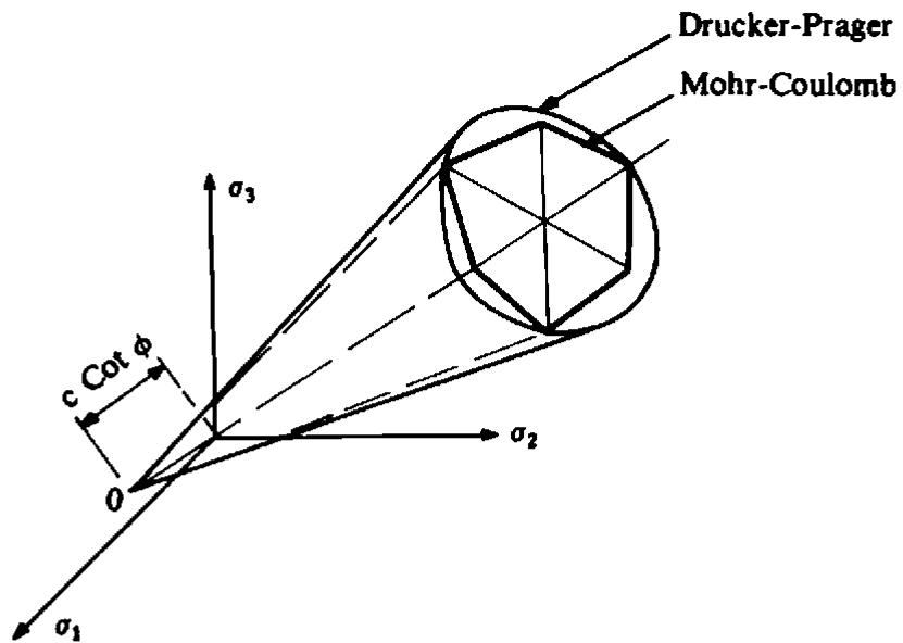
Fig. 7.4 (a) Geometrical representation of the Mohr-Coulomb and Drucker-Prager yield surfaces in principal stress space. 

text_image

σ₃ Mohr-Coulomb C B D 0 A θ E σ₁ F σ₂ Drucker-Prager Line of pure shear (θ = 0)

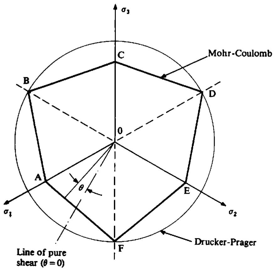
Fig. 7.4 (b) Two-dimensional, $\pi$ plane, representation of the Mohr-Coulomb and Drucker-Prager yield criteria. However, the approximation given by either the inner or outer cone to the true failure surface can be poor for certain stress combinations. $^{(5)}$ # 7.2.2 Work or strain hardening After initial yielding, the stress level at which further plastic deformation occurs may be dependent on the current degree of plastic straining. Such a phenomenon is termed work hardening or strain hardening. Thus the yield surface will vary at each stage of the plastic deformation, with the subsequent yield surfaces being dependent on the plastic strains in some way. Some alternative models which describe strain hardening in a material are illustrated in Fig. 7.5. A perfectly plastic material is shown in Fig. 7.5(a) where the yield stress level does not depend in any way on the degree of plastification. If the subsequent yield surfaces are a uniform expansion of the original yield curve, without translation, as shown in Fig. 7.5(b) the strain-hardening model is said to be isotropic. On the other hand if the subsequent yield surfaces preserve their shape and orientation but translate in the stress space as a rigid body as shown in Fig. 7.5(c), kinematic hardening is said to take place. Such a hardening model gives rise to the experimentally observed Bauschinger effect on cyclic loading.  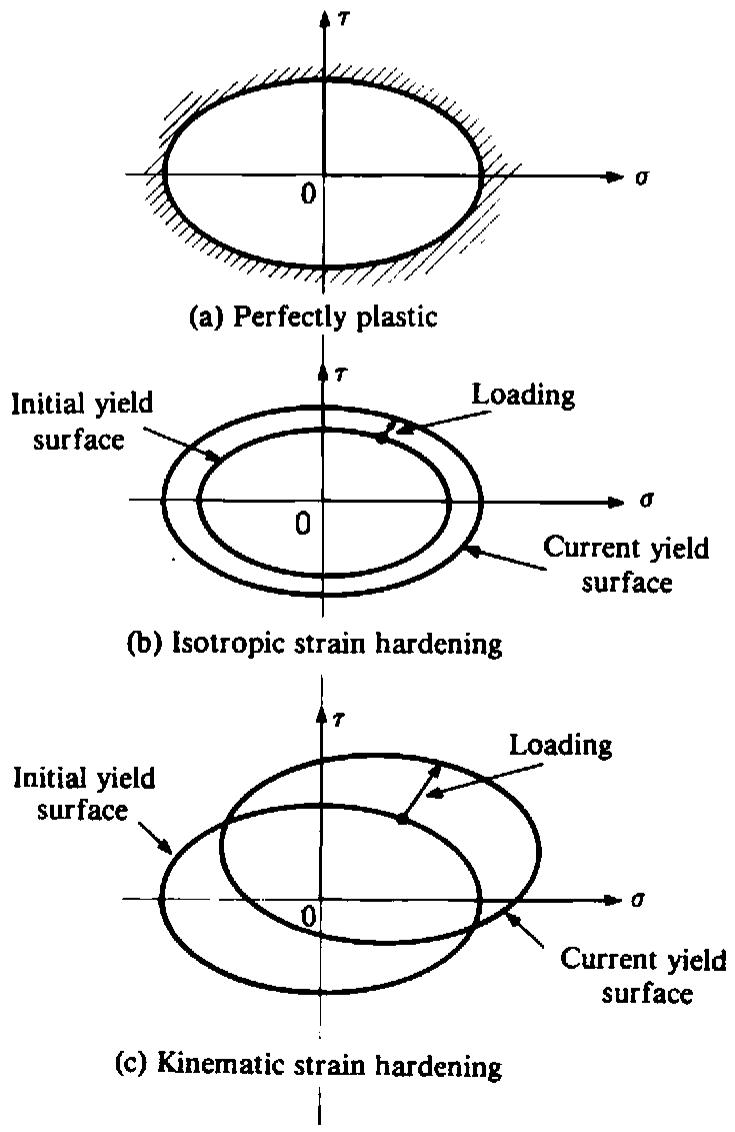Fig. 7.5 Mathematical models for representation of strain hardening behaviour. For some materials, notably soils, the yield surface may not strain harden but strain soften instead, so that the yield stress level at a point decreases with increasing plastic deformation. Therefore, for an isotropic model, the original yield curve contracts progressively without translation. Consequently yielding implies local failure and the yield surface becomes a failure criterion. The progressive development of the yield surface can be defined by relating the yield stress k to the plastic deformation by means of the hardening parameter $\kappa$ . This can be done in two ways. Firstly the degree of work hardening can be postulated to be a function of the total plastic work, $W_{p}$ , only. Then, $$ \kappa = W _ {p}, \tag {7.20} $$ where $$ W _ {p} = \int \sigma_ {i j} (d \epsilon_ {i j}) _ {p}, \tag {7.21} $$ in which $(d\epsilon_{ij})_{p}$ are the plastic components of strain occurring during a strain increment. Alternatively $\kappa$ can be related to a measure of the total plastic deformation termed the effective, generalised or equivalent plastic strain which is defined incrementally as $$ d \bar {\epsilon} _ {p} = \sqrt {\left(\frac {2}{3}\right)} \left\{\left(d \epsilon_ {i j}\right) _ {p} \left(d \epsilon_ {i j}\right) _ {p} \right\} ^ {\frac {1}{2}}. \tag {7.22} $$ A physical insight of this definition is provided in Section 7.2.4 where uniaxial yielding is considered. For situations where the assumption that yielding is independent of any hydrostatic stress is valid, $(d\epsilon_{ii})_{p}=0$ and hence $(d\epsilon_{ij}^{\prime})_{p}=(d\epsilon_{ij})_{p}$ . Consequently (7.22) can be rewritten as $$ d \bar {\epsilon} _ {p} = \sqrt {\left(\frac {2}{3}\right)} \left\{\left(d \epsilon_ {i j} ^ {\prime}\right) _ {p} \left(d \epsilon_ {i j} ^ {\prime}\right) _ {p} \right\} ^ {\frac {1}{2}}. \tag {7.23} $$ Then the hardening parameter, $\kappa$ , is assumed to be defined as $$ \kappa = \bar {\epsilon} _ {p}, \tag {7.24} $$ where $\bar{\epsilon}_{p}$ is the result of integrating $d\bar{\epsilon}_{p}$ over the strain path. This behaviour is termed strain hardening. Only an isotropic hardening model will be considered in this text. Stress states for which f = k represent plastic states, while elastic behaviour is characterised by f < k. At a plastic state, f = k, the incremental change in the yield function due to an incremental stress change is $$ d f = \frac {\partial f}{\partial \sigma_ {i j}} d \sigma_ {i j}. \tag {7.25} $$ Then if:- df<0 elastic unloading occurs (elastic behaviour) and the stress point returns inside the yield surface df=0 neutral loading (plastic behaviour for a perfectly plastic material) and the stress point remains on the yield surface df>0 plastic loading (plastic behaviour for a strain hardening material) and the stress point remains on the expanding yield surface. It can also be shown $^{(1-3)}$ that, for a stable material that the initial and all subsequent yield surfaces must be convex. # 7.2.3 Elasto-plastic stress/strain relation After initial yielding the material behaviour will be partly elastic and partly plastic. During any increment of stress, the changes of strain are assumed to be divisible into elastic and plastic components, so that $$ d \epsilon_ {i j} = (d \epsilon_ {i j}) _ {e} + (d \epsilon_ {i j}) _ {p}. \tag {7.26} $$ The elastic strain increment is related to the stress increment by (7.1). Or, decomposing the stress terms into their deviatoric and hydrostatic components $$ (d \epsilon_ {i j}) _ {e} = \frac {d \sigma_ {i j} ^ {\prime}}{2 \mu} + \frac {(1 - 2 \nu)}{E} \delta_ {i j} d \sigma_ {k k}, \tag {7.27} $$ where $E$ and $\nu$ are respectively the elastic modulus and Poisson's ratio of the material. In order to derive the relationship between the plastic strain component and the stress increment a further assumption on the material behaviour must be made. In particular it will be assumed that, the plastic strain increment is proportional to the stress gradient of a quantity termed the plastic potential Q, so that $$ (d \epsilon_ {i j}) _ {p} = d \lambda \frac {\partial Q}{\partial \sigma_ {i j}}, \tag {7.28} $$ where $d\lambda$ is a proportionality constant termed the plastic multiplier. A theoretical basis for this assumption is developed in Ref. 1. Equation (7.28) is termed the flow rule since it governs the plastic flow after yielding. The potential $Q$ must be a function of $J_2'$ and $J_3'$ but as yet it cannot be determined in its most general form. However the relation $f \equiv Q$ has a special significance in the mathematical theory of plasticity, since for this case certain variational principles and uniqueness theorems can be formulated. The identity $f \equiv Q$ is a valid one since it has been postulated that both are functions of $J_2'$ and $J_3'$ and such an assumption gives rise to an associated theory of plasticity. 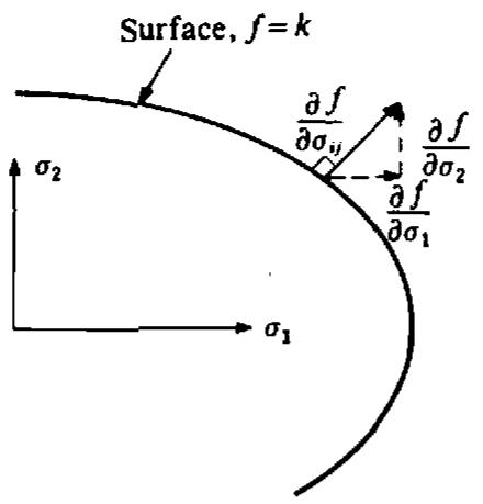In this case (7.28) becomes $$ (d \epsilon_ {i j}) _ {p} = d \lambda \frac {\partial f}{\partial \sigma_ {i j}}, \tag {7.29} $$ and is termed the normality condition since $\partial f / \partial \sigma_{ij}$ is a vector directed normal to the yield surface at the stress point under consideration as shown in Fig. 7.6. It is seen that the components of the plastic strain increment are required to combine vectorially in $n$ -dimensional space to give a vector 

text_image

Surface, f = k σ₂ ∂f/∂σᵢⱼ ∂f/∂σ₂ ∂f/∂σ₁ σ₁

Fig. 7.6 Geometrical representation of the normality rule of associated plasticity. which is normal to the yield surface. For the particular case of $f = J_{2}'$ we have $$ \frac {\partial f}{\partial \sigma_ {i j}} = \frac {\partial J _ {2} ^ {\prime}}{\partial \sigma_ {i j}} = \sigma_ {i j} ^ {\prime}. \tag {7.30} $$ Then (7.29) becomes $$ (d \epsilon_ {i j}) _ {p} = d \lambda \sigma_ {i j} ^ {\prime}, \tag {7.31} $$ which are known as the Prandtl–Reuss equations $^{(1)}$ and have been extensively employed in theoretical work. Experimental observations indicate that the normality condition is an acceptable assumption for metals, but the question of normality in rocks and soils is still open to debate $^{(6)}$ and is discussed further in Chapter 12. Thus on use of (7.26), (7.27) and (7.29) the complete incremental relationship between stress and strain for elasto-plastic deformation is found to be $$ d \epsilon_ {i j} = \frac {d \sigma_ {i j} ^ {\prime}}{2 \mu} + \frac {(1 - 2 \nu)}{E} \delta_ {i j} d \sigma_ {k k} + d \lambda \frac {\partial f}{\partial \sigma_ {i j}}. 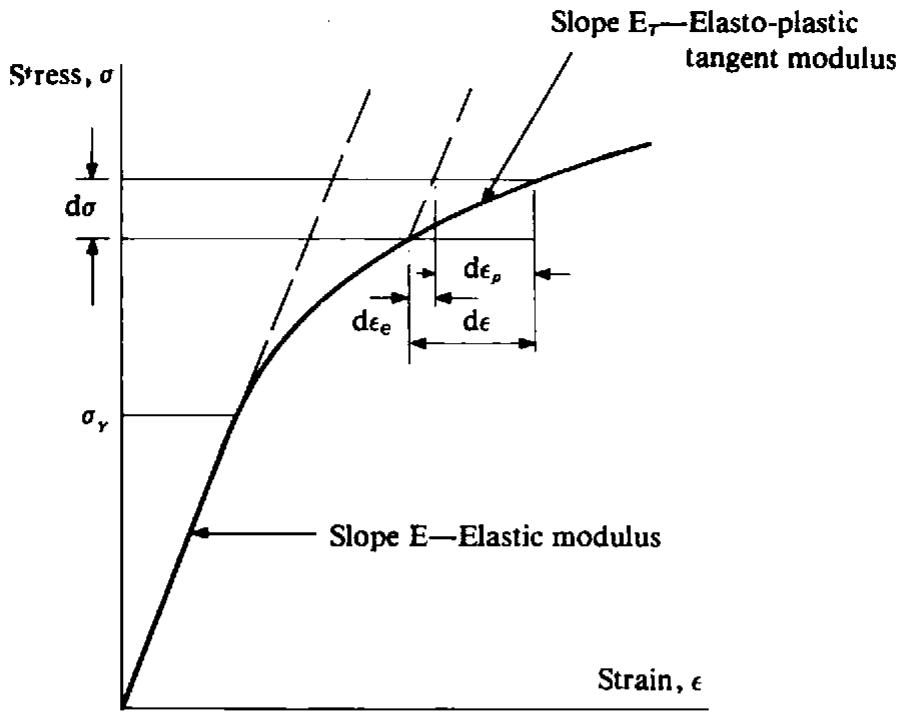\tag {7.32} $$ # 7.2.4 Uniaxial yield test on a strain-hardening material Consider the uniaxial testing of an elasto-plastic material which produces the stress-strain curve shown in Fig. 7.7. The behaviour is initially elastic characterised by an elastic modulus E until yielding commences at the uniaxial yield stress $\sigma_{Y}$ . Thereafter the material response is elasto-plastic with the local tangent to the curve continually varying and is termed the elasto-plastic tangent modulus, $E_{T}$ . The hardening law $k = k(\kappa)$ could just as easily be expressed in terms of the effective stress, $\bar{\sigma}$ (since it is proportional to $J_{2}'$ ) to give, for the strain hardening hypothesis (7.24) $$ \bar {\sigma} = H (\bar {\epsilon} _ {p}), \tag {7.33} $$ 

line

| Strain, ε | Stress, σ (Eτ-Elasto-plastic tangent modulus) | Stress, σ (E-Elastic modulus) | | --------- | --------------------------------------------- | ------------------------------ | | 0 | 0 | 0 | | ε | dσ | σγ | | εe | dεe | σγ | | ε | dεp | σγ | | εe | dεp | σγ |

Fig. 7.7 Elasto-plastic strain hardening behaviour for the uniaxial case. or differentiating, $$ \frac {d \bar {\sigma}}{d \bar {\epsilon} _ {p}} = H ^ {\prime} (\bar {\epsilon} _ {p}). \tag {7.34} $$ For the uniaxial case under consideration $\sigma_{1} = \sigma$ , $\sigma_{2} = \sigma_{3} = 0$ and thus from (7.12) $$ \bar {\sigma} = \sqrt {\left(\frac {3}{2}\right)} \{\sigma_ {i j} ^ {\prime} \sigma_ {i j} ^ {\prime} \} ^ {1 / 2} = \sigma . \tag {7.35} $$ If the plastic strain increment in the direction of loading is $d\epsilon_{p}$ , then $(d\epsilon_{1})_{p} = d\epsilon_{p}$ and since plastic straining is assumed to be incompressible, Poisson's ratio is effectively 0.5 and $(d\epsilon_{2})_{p} = -\frac{1}{2} d\epsilon_{p}$ and $(d\epsilon_{3})_{p} = -\frac{1}{2} d\epsilon_{p}$ . Then from (7.23) the effective plastic strain becomes $$ d \bar {\epsilon} _ {p} = \sqrt {\left(\frac {2}{3}\right)} \left\{\left(\epsilon_ {i j} ^ {\prime}\right) _ {p} \left(\epsilon_ {i j} ^ {\prime}\right) _ {p} \right\} ^ {1 / 2} = d \epsilon_ {p}. \tag {7.36} $$ Expressions (7.35) and (7.36) explain the apparent arbitrary constants employed in the definition of $\bar{\sigma}$ and $\bar{\epsilon}_{p}$ , since these terms are required to become the actual stress and strain for uniaxial yielding. Using (7.35) and (7.36) then (7.34) becomes $$ H ^ {\prime} (\bar {\epsilon} _ {p}) = \frac {d \sigma}{d \epsilon_ {p}} = \frac {d \sigma}{d \epsilon - d \epsilon_ {e}} = \frac {1}{d \epsilon / d \sigma - d \epsilon_ {e} / d \sigma}, $$ or $$ H ^ {\prime} = \frac {E _ {T}}{1 - E _ {T} / E}. \tag {7.37} $$ Thus the hardening function $H'$ can be determined experimentally from a simple uniaxial yield test. (For numerical computation it will be shown in the next section that it is $H'$ and not H that is required). # 7.3 Matrix formulation The theoretical expressions developed in Section 7.2 will now be converted to matrix form. $^{(7,8)}$ The yield function, first defined in (7.4), can be rewritten as $$ f (\sigma) = k (\kappa), \tag {7.38} $$ where $\sigma$ is the stress vector and $\kappa$ is the hardening parameter which governs the expansion of the yield surface. In particular, from (7.20) and (7.21), $d\kappa = \sigma^{T}d\epsilon_{p}$ for the work hardening hypothesis and from (7.24) $d\kappa = d\epsilon_{p}$ for the strain hardening hypothesis. Rearranging (7.38) we get $$ F (\sigma , \kappa) = f (\sigma) - k (\kappa) = 0. \tag {7.39} $$ By differentiating (7.39) we have $$ d F = \frac {\partial F}{\partial \sigma} d \sigma + \frac {\partial F}{\partial \kappa} d \kappa = 0, \tag {7.40} $$ or $$ \boldsymbol {a} ^ {T} d \sigma - A d \lambda = 0, \tag {7.41} $$ with the definitions $$ \boldsymbol {a} ^ {T} = \frac {\partial F}{\partial \sigma} = \left[ \frac {\partial F}{\partial \sigma_ {x}}, \frac {\partial F}{\partial \sigma_ {y}}, \frac {\partial F}{\partial \sigma_ {z}}, \frac {\partial F}{\partial \tau_ {y z}}, \frac {\partial F}{\partial \tau_ {z x}}, \frac {\partial F}{\partial \tau_ {x y}} \right], \tag {7.42} $$ and $$ A = - \frac {1}{d \lambda} \frac {\partial F}{\partial \kappa} d \kappa . \tag {7.43} $$ The vector a is termed the flow vector. Expression (7.32) can be immediately rewritten as $$ d \epsilon = [ D ] ^ {- 1} d \sigma + d \lambda \frac {\partial F}{\partial \sigma}, \tag {7.44} $$ where D is the usual matrix of elastic constants. Premultiplying both sides of (7.44) by $d_{D}^{T} = a^{T}D$ and eliminating $a^{T}d\sigma$ by use of (7.41) we obtain the plastic multiplier $d\lambda$ to be $$ d \lambda = \frac {1}{[ A + a ^ {T} D a ]} a ^ {T} d _ {D} d \epsilon . \tag {7.45} $$ Or substituting (7.45) into (7.44) we obtain the complete elasto-plastic incremental stress-strain relation to be $$ d \sigma = D _ {e p} d \epsilon , \tag {7.46} $$ with $$ \boldsymbol {D} _ {e p} = \boldsymbol {D} - \frac {\boldsymbol {d} _ {D} \boldsymbol {d} _ {D} ^ {T}}{\boldsymbol {A} + \boldsymbol {d} _ {0} ^ {T} \boldsymbol {a}}; \quad \boldsymbol {d} _ {D} = \boldsymbol {D} \boldsymbol {a}. \tag {7.47} $$ This expression for $D_{ep}$ is similar in form to that for one dimensional application given in Page 28, Chapter 2. It now remains to determine the explicit form of the scalar term, A. The work hardening hypothesis is more general from a thermodynamic viewpoint $^{(9)}$ than the strain hardening hypothesis and will be employed for numerical work in this text. Therefore $$ d \kappa = \sigma^ {T} d \epsilon_ {p}. \tag {7.48} $$ Equation (7.39) can be rewritten in the form $$ F (\sigma , \kappa) = f (\sigma) - \sigma_ {Y} (\kappa) = 0, \tag {7.49} $$ since the uniaxial yield stress, $\sigma_{Y} = \sqrt{(3)} k$ . Thus from (7.43) $$ A = - \frac {1}{d \lambda} \frac {\partial F}{\partial \kappa} d \kappa = \frac {1}{d \lambda} \frac {d \sigma_ {Y}}{d \kappa} d \kappa . \tag {7.50} $$ Note that the full differential may be employed in the last term since $\sigma_{Y}$ is a function of $\kappa$ only. Employing the normality condition in (7.48) to express $d\epsilon_{p}$ we have $$ d \kappa = \sigma^ {T} d \epsilon_ {p} = \sigma^ {T} d \lambda a = d \lambda a ^ {T} \sigma . \tag {7.51} $$ Or, for the uniaxial case $\sigma = \bar{\sigma} = \sigma_{Y}$ and $d\epsilon_{p} = d\bar{\epsilon}_{p}$ where $\bar{\sigma}$ and $\bar{\epsilon}_{p}$ are respectively the effective stress and strain. Thus (7.51) becomes $$ d \kappa = \sigma_ {Y} d \bar {\epsilon} _ {p} = d \lambda a ^ {T} \sigma . \tag {7.52} $$ Also, from (7.34) we have $$ \frac {d \bar {\sigma}}{d \bar {\epsilon} _ {p}} = \frac {d \sigma_ {Y}}{d \bar {\epsilon} _ {p}} = H ^ {\prime}. \tag {7.53} $$ Using Euler's theorem† applicable to all homogeneous functions of order one, we can write from (7.49) $$ \frac {\partial f}{\partial \sigma} \sigma = \sigma_ {Y}. \tag {7.54} $$ Or from (7.42) $$ \boldsymbol {a} ^ {T} \boldsymbol {\sigma} = \sigma_ {Y}. \tag {7.55} $$ Substituting (7.53) and (7.55) into (7.52) and (7.50) we obtain $$ d \lambda = d \bar {\epsilon} _ {p} $$ $$ A = H ^ {\prime}. \tag {7.56} $$ † Euler's theorem on homogeneous functions states that if $f(\mathbf{x})$ is homogeneous and of degree $n$ then $(\partial f / \partial \mathbf{x})$ . $\mathbf{x} = nf$ . Thus A is obtained to be the local slope of the uniaxial stress/plastic strain curve and can be determined experimentally from (7.37). # 7.4 Alternative form of the yield criteria for numerical computation For numerical computations it is convenient to rewrite the yield function in terms of alternative stress invariants. This formulation is due to Nayak $^{(10)}$ and its main advantage is that it permits the computer coding of the yield function and the flow rule in a general form and necessitates only the specification of three constants for any individual criterion. The principal deviatoric stresses $\sigma_{1}^{\prime}$ , $\sigma_{2}^{\prime}$ , $\sigma_{3}^{\prime}$ are given as the roots of the cubic equation $^{(11)}$ $$ t ^ {3} - J _ {2} ^ {\prime} t - J _ {3} ^ {\prime} = 0. \tag {7.57} $$ Noting the trigonometric identity $$ \sin^ {3} \theta - \frac {3}{4} \sin \theta + \frac {1}{4} \sin 3 \theta = 0, \tag {7.58} $$ and substituting $t = r \sin \theta$ into (7.57) we have $$ \sin^ {3} \theta - \frac {J _ {2} ^ {\prime}}{r ^ {2}} \sin \theta - \frac {J _ {3} ^ {\prime}}{r ^ {3}} = 0. \tag {7.59} $$ Comparing (7.58) and (7.59) gives $$ r = \frac {2}{\sqrt {3}} (J _ {2} ^ {\prime}) ^ {1 / 2}, \tag {7.60} $$ $$ \sin 3 \theta = - \frac {4 J _ {3} ^ {\prime}}{r ^ {3}} = - \frac {3 \sqrt {3}}{2} \frac {J _ {3} ^ {\prime}}{\left(J _ {2} ^ {\prime}\right) ^ {3 / 2}}. \tag {7.61} $$ The first root of (7.61) with $\theta$ determined for $3\theta$ in the range $\pm\pi/2$ is a convenient alternative to the third invariant, $J_{3}^{\prime}$ . By noting the cyclic nature of $\sin(3\theta+2n\pi)$ we have immediately the three (and only three) possible values of $\sin\theta$ which define the three principal stresses. The deviatoric principal stresses are given by $t=r\sin\theta$ on substitution of the three values of $\sin\theta$ in turn. Substituting for $r$ from (7.60) and adding the mean hydrostatic stress component gives the total principal stresses to be $$ \left\{ \begin{array}{l} \sigma_ {1} \\ \sigma_ {2} \\ \sigma_ {3} \end{array} \right\} = \frac {2 \left(J _ {2} ^ {\prime}\right) ^ {\frac {1}{2}}}{\sqrt {3}} \left\{ \begin{array}{l} \sin \left(\theta + \frac {2 \pi}{3}\right) \\ \sin \theta \\ \sin \left(\theta + \frac {4 \pi}{3}\right) \end{array} \right\} + \frac {J _ {1}}{3} \left\{ \begin{array}{l} 1 \\ 1 \\ 1 \end{array} \right\}, \tag {7.62} $$ with $\sigma_{1} > \sigma_{2} > \sigma_{3}$ and $-\pi / 6 \leqslant \theta \leqslant \pi / 6$ . The term $\theta$ is essentially similar to the Lode parameter(1) $\Gamma$ defined by $\Gamma = -\sqrt{(3)} \tan \theta$ . The four yield criteria considered in Section 7.2.1 can now be rewritten in terms of $J_{1}, J_{2}'$ and $\theta$ as follows. The Tresca yield criterion Substitute for $\sigma_{1}$ and $\sigma_{3}$ from (7.62) into (7.8) gives $$ \frac {2}{\sqrt {3}} (J _ {2} ^ {\prime}) ^ {\frac {1}{2}} \left[ \sin \left(\theta + \frac {2 \pi}{3}\right) - \sin \left(\theta + \frac {4 \pi}{3}\right) \right] = Y (\kappa), $$ or expanding we have $$ 2 (J _ {2} ^ {\prime}) ^ {\frac {1}{2}} \cos \theta = Y (\kappa) = \sqrt {(3)} k (\kappa) = \sigma_ {Y} (\kappa). \tag {7.63} $$ The physical interpretation of $\theta$ is evident from Fig. 7.2. The Von Mises yield criterion There is no change in this case since this yield function depends on $J_2'$ only. From (7.9) $$ (J _ {2} ^ {\prime}) ^ {\frac {1}{2}} = k (\kappa), $$ or $\sqrt{3}(J_2')^{\frac{1}{2}} = \sigma_Y(\kappa).$ (7.64) The Mohr-Coulomb yield criterion Substituting from (7.62) for $\sigma_{1}$ and $\sigma_{3}$ into (7.16) results in $$ \frac {1}{3} J _ {1} \sin \phi + (J _ {2} ^ {\prime}) ^ {1 / 2} \left(\cos \theta - \frac {1}{\sqrt {3}} \sin \theta \sin \phi\right) = c \cos \phi . \tag {7.65} $$ The Drucker-Prager yield criterion There is no change for this criterion and we can write directly from (7.17) that $$ a J _ {1} + (J _ {2} ^ {\prime}) ^ {\frac {1}{2}} = k ^ {\prime}, \tag {7.66} $$ where $a$ and $k'$ are defined in (7.18) or (7.19). In order to calculate the $D_{ep}$ matrix in (7.47) we require to express the flow vector a in a form suitable for numerical computation. We can always write $$ \boldsymbol {a} ^ {T} = \frac {\partial F}{\partial \sigma} = \frac {\partial F}{\partial J _ {1}} \frac {\partial J _ {1}}{\partial \sigma} + \frac {\partial F}{\partial (J _ {2} ^ {\prime}) ^ {1 / 2}} \frac {\partial (J _ {2} ^ {\prime}) ^ {1 / 2}}{\partial \sigma} + \frac {\partial F}{\partial \theta} \frac {\partial \theta}{\partial \sigma}, \tag {7.67} $$ where $$ \sigma^ {T} = \left\{\sigma_ {x}, \sigma_ {y}, \sigma_ {z}, \tau_ {y z}, \tau_ {z x}, \tau_ {x y} \right\}. $$ Differentiating (7.61) we obtain $$ \frac {\partial \theta}{\partial \sigma} = \frac {- \sqrt {3}}{2 \cos 3 \theta} \left[ \frac {1}{(J _ {2} ^ {\prime}) ^ {3 / 2}} \frac {\partial J _ {3}}{\partial \sigma} - \frac {3 J _ {3}}{(J _ {2} ^ {\prime}) ^ {2}} \frac {\partial (J _ {2} ^ {\prime}) ^ {1 / 2}}{\partial \sigma} \right]. \tag {7.68} $$ Substituting this in (7.67) and using (7.61), we can then write