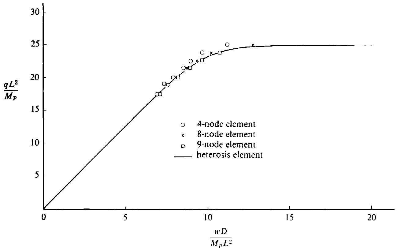
Typical input for the nonlayered approach is given in Appendix IV together with lineprinter output of results. Figures 9.7 and 9.8 show the load displacement curves for both layered and nonlayered approaches. 

line

| wD / (MpL²) | 4-node element | 8-node element | 9-node element | heterosis element | | ----------- | -------------- | -------------- | -------------- | ----------------- | | 0 | 0 | 0 | 0 | 0 | | 7 | 17.5 | 17.5 | 17.5 | 17.5 | | 8 | 20.0 | 20.0 | 20.0 | 20.0 | | 9 | 22.0 | 22.0 | 22.0 | 22.0 | | 10 | 23.5 | 23.5 | 23.5 | 23.5 | | 11 | 24.5 | 24.5 | 24.5 | 24.5 | | 12 | 24.8 | 24.8 | 24.8 | 24.8 | | 13 | 24.9 | 24.9 | 24.9 | 24.9 | | 14 | 24.95 | 24.95 | 24.95 | 24.95 | | 15 | 24.98 | 24.98 | 24.98 | 24.98 | | 16 | 24.99 | 24.99 | 24.99 | 24.99 | | 17 | 24.995 | 24.995 | 24.995 | 24.995 | | 18 | 24.998 | 24.998 | 24.998 | 24.998 | | 19 | 24.999 | 24.999 | 24.999 | 24.999 | | 20 | 25.0 | 25.0 | 25.0 | 25.0 |

Fig. 9.7 Load displacement curves for nonlayered approach. 

line

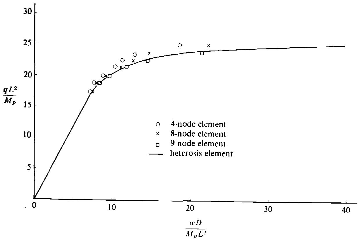
| wD / (Mp L²) | 4-node element | 8-node element | 9-node element | heterosis element | | ------------ | -------------- | -------------- | -------------- | ----------------- | | 0 | 0 | 0 | 0 | 0 | | 5 | 17 | 17 | 18 | 17 | | 10 | 20 | 20 | 20 | 20 | | 15 | 22 | 22 | 22 | 22 | | 20 | 24 | 24 | 23 | 23 | | 25 | 24 | 24 | 23 | 23 | | 30 | 24 | 24 | 23 | 23 | | 35 | 24 | 24 | 23 | 23 | | 40 | 24 | 24 | 23 | 23 |

Fig. 9.8 Load displacement curves for layered approach. 

text_image

y L -∞← -∞ x

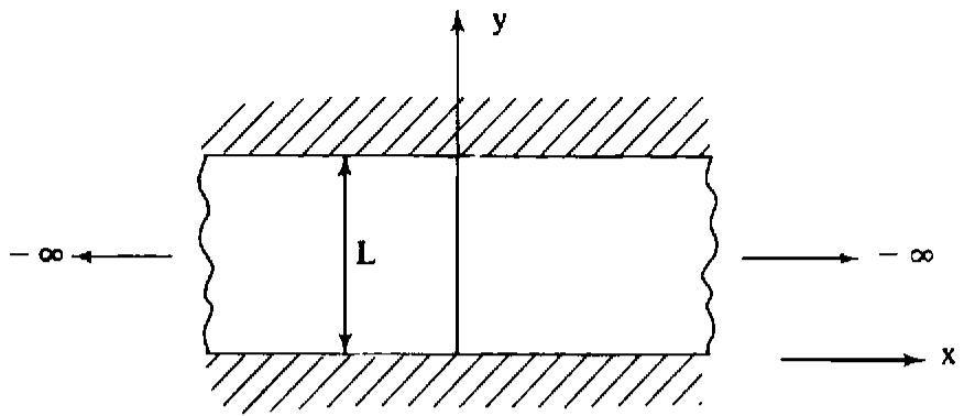
Fig. 9.9 Infinite clamped plate strip under uniform lateral load q. # 9.8 Problems 9.1 Consider the uniformly loaded, clamped plate shown in Fig. 9.9. Using programs MINDLIN and MINDLAY find the collapse load for the plate which has the following properties: Elastic modulus $E = 10000.0$ , Poisson's ratio $\nu = 0.3$ , thickness $t = 0.01$ , length $L = 1.00$ and yield stress $\sigma_0 = 1000.0$ . Check your solution using program PLANET. 9.2 Use program MINDLIN to find the value of the uniformly distributed load intensity q at which yielding first occurs for rectangular, simply supported plates of aspect ratios 1.0, 1.2, 1.4, 1.6, 2.0 and 2.2. Assume a thickness/span ratio of 0.05 and locate also the position of first yielding. Compare your results with those of Turvey $^{(9)}$ for a Von Mises material. 9.3 Modify program MINDLAY to allow for in-plane deformation of the plate mid-plane. Use a displacement pattern of the form $$ u (x, y, z) = u _ {0} (x, y) - z \theta_ {x} (x, y) \tag {9.31} $$ $$ v (x, y, z) = v _ {0} (x, y) - z \theta_ {y} (x, y) \tag {9.32} $$ in which $u_{0}$ and $v_{0}$ are the in-plane deflections of the plate mid-plane in the x and y directions respectively. 9.4 Modify programs MINDLIN and MINDLAY to allow for an elastic Winkler foundation of modulus K. The appropriate virtual work term is $$ \int_ {\Omega} \delta w K w d \Omega $$ in which $\delta w$ is the virtual lateral displacement. 9.5 Solve the beam problem in Example 5.1 of Chapter 5 using programs MINDLIN and MINDLAY. 9.6 Develop a program for the nonlayered elastoplastic analysis of axisymmetric Mindlin plates using 2-node radial finite elements. The virtual work expression for an annular plate of internal and external radii $r_{0}$ and $r_{1}$ respectively is given as $$ \begin{array}{l} 2 \pi \int_ {r _ {0}} ^ {r _ {1}} \left[ - \frac {d (\delta \theta)}{d r} M _ {r} - \frac {\delta \theta}{r} M _ {\theta} + \left(\frac {d (\delta w)}{d r} - \theta\right) Q \right] r d r \\ - 2 \pi \int_ {r _ {0}} ^ {r _ {1}} \delta w q r d r \tag {9.33} \\ \end{array} $$ in which the radial bending moment $M_{r} = -D[d\theta/dr + \nu\theta/r]$ the circumferential bending moment $M_{\theta} = -D[\theta/r + \nu d\theta/dr]$ the shear force $Q = [Gt(dw/dr - \theta)]/1.2$ , $\theta$ is the normal rotation in the radial rz plane and w is the lateral displacement in the z direction. # 9.9 References 1. HUGHES, T. J. R. and COHEN, M., The 'Heterosis' finite element for plate bending, Computers and Structures 9, 445–450 (1978). 2. BHAUMIK, A. K. and HANLEY, J. T., Elasto-plastic plate analysis by finite differences, J. Struct. Div. ASCE, 93, 575 (1967). 3. ARMEN, H., PIFKO, A. and LEVINE, H. S., A finite element method for the plastic bending analysis of structures, Proc. of the Second Conf. on Matrix Methods in Struct. Mech., Wright-Patterson Air Force Base, Dayton, Ohio, 1301-1339 (1968). 4. LOPEZ, L. A. and ANG, A. H. I., Flexural analysis of elastic-plastic rectangular plates, Civil Engineering Studies, Structural Research Series No. 305, University of Illinois (1966). 5. McNIECE, G. M. and KEMP, K. O., Comparison of finite element and unique limit analysis solutions for certain reinforced concrete slabs. Proc. Instn. Civ. Engrs. 43, 629–640 (1969). 6. BACKLUND, J., Mixed finite element analysis of elastic and elasto-plastic plates in bending, Chalmers University of Technology, Department of Structural Mechanics, Publication 71: 1, 30, Göteborg (1971). 7. WEGMULLER, A. W. and KOSTEM, C. N., Finite element analysis of elastic-plastic plates and eccentrically stiffened plates, Fritz Engineering Laboratory Report No. 376A4, Lehigh University, Bethlehem, Pennsylvania (1973). 8. HINTON, E. and OWEN, D. R. J., Finite Element Programming, Academic Press (1977). 9. TURVEY, G. J., First yield analysis of laterally loaded, rectangular, Levy plates with unsymmetric, side boundary conditions, Proc. Instn. Civ. Engrs., 65, 199–206 (1978). # Part III # Chapter 10 Explicit transient dynamic analysis Written in collaboration with D. K. Paul and N. Bicanic # 10.1 Introduction Earlier, in Parts I and II, we considered static (or pseudostatic) applications. However, many structures are subjected to time-varying loads such as impulse, blast, impact or earthquake loading. Here in Part III we consider finite element based methods for dealing with such problems. Although a form of mode-superposition has been adopted in nonlinear transient dynamic stress analysis, $^{(1)}$ it is general practice to use a time stepping procedure. Such direct integration schemes may be broadly classified as either explicit or implicit methods. In the present chapter, we consider the very popular and easily implemented, explicit, central difference scheme. During each time step, relatively little computational effort is required since no formal matrix factorisation is necessary. Unfortunately, the method is conditionally stable and very small time steps are often needed. In implicit schemes, a matrix factorisation is required but we can select an unconditionally stable implicit algorithm in which the time step length is governed by considerations of accuracy alone. In Chapter 11 we consider the Newmark family $^{(2)}$ of time stepping schemes. We then present a program for nonlinear transient dynamic stress analysis in which we may select any of the following algorithms: (i) an implicit solution (ii) an explicit solution (iii) a combined implicit/explicit solution The programs in Chapters 10 and 11 deal with plane stress, plane strain and axisymmetric applications using 4, 8 and 9-node, isoparametric quadrilaterals. Geometrically nonlinear behaviour is taken into account using a Total Lagrangian formulation. In Chapter 10 the material behaviour is assumed to be elasto-viscoplastic, whereas an elasto-plastic model is used in Chapter 11. Test examples are presented for both programs. # 10.2 Dynamic equilibrium equations For dynamic equilibrium of a body in motion we can use the Principle of Virtual Work to write the following equations at time station $t_{n}$ irrespective of material behaviour $$ \begin{array}{l} \int_ {\Omega} \left[ \delta \boldsymbol {\epsilon} _ {n} \right] ^ {T} \boldsymbol {\sigma} _ {n} d \Omega - \int_ {\Omega} \left[ \delta \boldsymbol {u} _ {n} \right] ^ {T} \left[ \boldsymbol {b} _ {n} - \rho_ {n} \ddot {\boldsymbol {u}} _ {n} - c _ {n} \dot {\boldsymbol {u}} _ {n} \right] d \Omega \\ - \int_ {\Gamma_ {t}} \left[ \delta \boldsymbol {u} _ {n} \right] ^ {T} \boldsymbol {t} _ {n} d \Gamma = 0 \tag {10.1} \\ \end{array} $$ where $\delta u_{n}$ is the vector of virtual displacements, $\delta \epsilon_{n}$ is the vector of associated virtual strains, $b_{n}$ is the vector of applied body forces, $t_{n}$ is the vector of surface tractions, $\sigma_{n}$ is the vector of stresses, $\rho_{n}$ is the mass density, $c_{n}$ is the damping parameter and a dot refers to differentiation with respect to time. The domain of interest $\Omega$ has two boundaries: $\Gamma_{t}$ on which boundary tractions $t_{n}$ are specified and $\Gamma_{u}$ on which displacements $u_{n}$ are specified. For plane stress, plane strain and axisymmetric problems all of these terms were defined in Chapter 6. Recall that in Chapter 6 we noted that, for a finite element representation, the displacements and strains and also their virtual counterparts are given by the relationships $$ \pmb {u} _ {n} = \sum_ {i = 1} ^ {m} N _ {i} [ \pmb {d} _ {i} ] _ {n}, \qquad \delta \pmb {u} _ {n} = \sum_ {i = 1} ^ {m} N _ {i} [ \delta \pmb {d} _ {i} ] _ {n} \tag {10.2} $$ $$ \epsilon_ {n} = \sum_ {i = 1} ^ {m} B _ {i} [ d _ {i} ] _ {n}, \quad \delta \epsilon_ {n} = \sum_ {i = 1} ^ {m} B _ {i} [ \delta d _ {i} ] _ {n} \tag {10.3} $$ where at time station $t_{n}$ for node i, $[d_{i}]_{n}$ is the vector of nodal displacements, $[\delta d_{i}]_{n}$ is the vector of virtual nodal variables, $N_{i} = N_{i}I_{2}$ is the matrix of global shape functions and $B_{i}$ is the global strain-displacement matrix. $^{\dagger}$ The total number of nodes is m. If (10.2) and (10.3) are substituted into (10.1), and if we note that the resulting equation is true for any set of virtual displacements $[\delta d]_{n}$ then we obtain for each node i the equations. $$ [ p _ {i} ] _ {n} - [ f _ {B i} ] _ {n} + [ f _ {I i} ] _ {n} + [ f _ {D i} ] _ {n} - [ f _ {T i} ] _ {n} = 0 \tag {10.4} $$ where the internal resisting forces are $$ [ \pmb {p} _ {i} ] _ {n} = \int_ {\Omega} [ \pmb {B} _ {i} ] ^ {T} \pmb {\sigma} _ {n} d \Omega , \tag {10.5} $$ the consistent forces for the applied body forces are $$ [ \pmb {f} _ {B i} ] _ {n} = \int_ {\Omega} [ N _ {i} ] ^ {T} \pmb {b} _ {n} d \Omega , \tag {10.6} $$ the inertia forces are $$ \begin{array}{l} \left[ \boldsymbol {f} _ {I i} \right] _ {n} = \int_ {\Omega} \left[ \boldsymbol {N} _ {i} \right] ^ {T} \rho_ {n} \left[ \boldsymbol {N} _ {1}, \boldsymbol {N} _ {2}, \dots , \boldsymbol {N} _ {m} \right] d \Omega \left[ \begin{array}{c} \left[ \ddot {\boldsymbol {d}} _ {1} \right] _ {n} \\ \left[ \ddot {\boldsymbol {d}} _ {2} \right] _ {n} \\ \vdots \end{array} \right] \tag {10.7} \\ = \sum_ {j = 1} ^ {m} [ \boldsymbol {M} _ {i j} ] _ {n} [ \ddot {\boldsymbol {d}} _ {j} ] _ {n}, \quad \left\lfloor \quad [ \ddot {\boldsymbol {d}} _ {m} ] _ {n} \right. \\ \end{array} $$ (N.B. $[M_{ij}]_{n}$ is a submatrix of the mass matrix $M_{n}$ ) The damping forces are $$ \begin{array}{l} \left[ \boldsymbol {f} _ {D i} \right] _ {n} = \int_ {\Omega} \left[ \boldsymbol {N} _ {i} \right] ^ {T} c _ {n} \left[ \boldsymbol {N} _ {1}, \boldsymbol {N} _ {2}, \dots , \boldsymbol {N} _ {m} \right] d \Omega \\ = \sum_ {j = 1} ^ {m} \left[ \boldsymbol {C} _ {i j} \right] _ {n} \left[ \dot {\boldsymbol {d}} _ {j} \right] _ {n} \end{array} \left[ \begin{array}{c} \left[ \dot {\boldsymbol {d}} _ {1} \right] \\ \left[ \dot {\boldsymbol {d}} _ {2} \right] \\ \vdots \\ \left[ \dot {\boldsymbol {d}} _ {m} \right] \end{array} \right] \tag {10.8} $$ (N.B. $[C_{ij}]_{n}$ is a submatrix of the damping matrix $C_{n}$ ) and the consistent forces for the traction boundary forces are $$ [ f _ {T i} ] _ {n} = \int_ {\Gamma_ {r}} [ N _ {i} ] ^ {T} t _ {n} d \Gamma . \tag {10.9} $$ If we use $C(0)$ isoparametric finite element representations we can evaluate contributions to (10.4) separately from each element and then assemble them into the appropriate vectors in (10.4). As noted in Chapter 6 the displacements can be expressed in the usual way as $$ [ \boldsymbol {u} ^ {(e)} ] _ {n} = \sum_ {i = 1} ^ {r} N _ {i} ^ {(e)} [ \boldsymbol {d} _ {i} ^ {(e)} ] _ {n} \tag {10.10} $$ where for local node i of element e, $N_{i}^{(e)} = N_{i}^{(e)}I_{2}$ is the local shape function matrix and $[d_{i}^{(e)}]_{n}$ is the vector of nodal displacements. As described in Chapter 6 we use 4, 8 and 9 noded isoparametric quadrilateral elements and therefore $r = 4, 8$ and 9 respectively for these cases. The strain displacement relationships are expressed as $$ [ \epsilon^ {(e)} ] _ {n} = \sum_ {i = 1} ^ {r} B _ {i} ^ {(e)} [ d _ {i} ^ {(e)} ] _ {n} \tag {10.11} $$ in which $\boldsymbol{B}_{t}^{(e)}$ is the local element strain matrix which has been defined for the various applications in Table 6.1. The discretised elemental volume is given as $$ d \Omega^ {(e)} = h ^ {(e)} \det J ^ {(e)} d \xi d \eta \tag {10.12} $$ in which $\det J^{(e)}$ is the determinant of the Jacobian matrix and $h^{(e)}$ is defined in Chapter 6. Thus the element contributions to the terms in (10.4) may be evaluated using numerical integration based on Gauss-Legendre product rules. These contributions now take the form $$ [ p _ {i} ^ {(e)} ] _ {n} = \int_ {- 1} ^ {+ 1} \int_ {- 1} ^ {+ 1} [ B _ {i} ^ {(e)} ] ^ {T} \sigma_ {n} ^ {(e)} h ^ {(e)} \det J ^ {(e)} d \xi d \eta \tag {10.13} $$ $$ [ f _ {B i} ^ {(e)} ] _ {n} = \int_ {- 1} ^ {+ 1} \int_ {- 1} ^ {+ 1} [ N _ {i} ^ {(e)} ] ^ {T} b _ {n} h ^ {(e)} \det J ^ {(e)} d \xi d \eta \tag {10.14} $$ $$ \begin{array}{l} \left[ f _ {I t} ^ {(e)} \right] _ {n} = \int_ {- 1} ^ {+ 1} \int_ {- 1} ^ {+ 1} \left[ N _ {t} ^ {(e)} \right] ^ {T} \rho_ {n} ^ {(e)} \left[ N _ {1} ^ {(e)}, N _ {2} ^ {(e)}, \dots , N _ {r} ^ {(e)} \right] h ^ {(e)} \det J ^ {(e)} d \xi d \eta \left[ \begin{array}{c} \left[ \ddot {d} _ {1} ^ {(e)} \right] _ {n} \\ \cdot \\ \cdot \\ \left[ \ddot {d} _ {r} ^ {(e)} \right] _ {n} \end{array} \right] \\ = \sum_ {j = 1} ^ {r} \left[ M _ {i j} ^ {(e)} \right] _ {n} \left[ \ddot {d} _ {j} ^ {(e)} \right] _ {n} \tag {10.15} \\ \end{array} $$ $$ \left[ f _ {D i} ^ {(e)} \right] _ {n} = \int_ {- 1} ^ {+ 1} \int_ {- 1} ^ {+ 1} \left[ N _ {i} ^ {(e)} \right] ^ {T} c _ {n} ^ {(e)} \left[ N _ {1} ^ {(e)}, N _ {2} ^ {(e)}, \dots , N _ {r} ^ {(e)} \right] h ^ {(e)} \det J ^ {(e)} d \xi d \eta \left[ \begin{array}{c} \left[ \dot {d} _ {1} ^ {(e)} \right] _ {n} \\ \cdot \\ \cdot \\ \cdot \\ \left[ \dot {d} _ {r} ^ {(e)} \right] _ {n} \end{array} \right] $$ $$ = \sum_ {j = 1} ^ {r} \left[ C _ {i j} ^ {(e)} \right] _ {n} \left[ \dot {\boldsymbol {d}} _ {j} ^ {(e)} \right] _ {n} \tag {10.16} $$ $$ [ f _ {T t ^ {(e)}} ] _ {n} = \int_ {\Gamma_ {t} ^ {(e)}} [ N _ {t ^ {(e)}} ] ^ {T} t _ {n} ^ {(e)} d \Gamma \tag {10.17} $$ where $\Gamma_{t}^{(e)}$ (if it exists) is that part of $\Gamma_{t}$ which coincides with the boundary of element domain $\Omega^{(e)}$ .