$$ \underline {{k}} ^ {(1)} = \left[ \begin{array}{c c} 1 & 3 \\ 1 0 0 0 & - 1 0 0 0 \\ - 1 0 0 0 & 1 0 0 0 \end{array} \right] \begin{array}{l} 1 \\ 3 \end{array} \quad \underline {{k}} ^ {(2)} = \left[ \begin{array}{c c} 3 & 4 \\ 2 0 0 0 & - 2 0 0 0 \\ - 2 0 0 0 & 2 0 0 0 \end{array} \right] \begin{array}{l} 3 \\ 4 \end{array} \tag {2.5.16} $$ $$ \underline {{k}} ^ {(3)} = \left[ \begin{array}{c c} 3 0 0 0 & - 3 0 0 0 \\ - 3 0 0 0 & 3 0 0 0 \end{array} \right] \begin{array}{c} 4 \\ 2 \end{array} $$ where the numbers above the columns and next to each row indicate the nodal degrees of freedom associated with each element. For instance, element 1 is associated with degrees of freedom $d _ { 1 x }$ and $d _ { 3 x }$ . Also, the local x^ axis coincides with the global x axis for each element. Using the concept of superposition (the direct stiffness method), we obtain the global stiffness matrix as $$ \underline {{K}} = \underline {{k}} ^ {(1)} + \underline {{k}} ^ {(2)} + \underline {{k}} ^ {(3)} $$ $$ \text { or } \quad \underline {{K}} = \left[ \begin{array}{c c c c} 1 & 2 & 3 & 4 \\ 1 0 0 0 & 0 & - 1 0 0 0 & 0 \\ 0 & 3 0 0 0 & 0 & - 3 0 0 0 \\ - 1 0 0 0 & 0 & 1 0 0 0 + 2 0 0 0 & - 2 0 0 0 \\ 0 & - 3 0 0 0 & - 2 0 0 0 & 2 0 0 0 + 3 0 0 0 \end{array} \right] \begin{array}{l} 1 \\ 2 \\ 3 \\ 4 \end{array} \tag {2.5.17} $$ (b) The global stiffness matrix, Eq. (2.5.17), relates global forces to global displacements as follows: $$ \left\{ \begin{array}{l} F _ {1 x} \\ F _ {2 x} \\ F _ {3 x} \\ F _ {4 x} \end{array} \right\} = \left[ \begin{array}{c c c c} 1 0 0 0 & 0 & - 1 0 0 0 & 0 \\ 0 & 3 0 0 0 & 0 & - 3 0 0 0 \\ - 1 0 0 0 & 0 & 3 0 0 0 & - 2 0 0 0 \\ 0 & - 3 0 0 0 & - 2 0 0 0 & 5 0 0 0 \end{array} \right] \left\{ \begin{array}{l} d _ {1 x} \\ d _ {2 x} \\ d _ {3 x} \\ d _ {4 x} \end{array} \right\} \tag {2.5.18} $$ Applying the homogeneous boundary conditions $d _ { 1 x } = 0$ and $d _ { 2 x } = 0$ t o Eq. (2.5.18), substituting applied nodal forces, and partitioning the first two equations of Eq. (2.5.18) (or deleting the first two rows of $\{ F \}$ and $\{ d \}$ and the first two rows and columns of $\underline { { K } }$ corresponding to the zero-displacement boundary conditions), we obtain $$ \left\{ \begin{array}{c} 0 \\ 5 0 0 0 \end{array} \right\} = \left[ \begin{array}{c c} 3 0 0 0 & - 2 0 0 0 \\ - 2 0 0 0 & 5 0 0 0 \end{array} \right] \left\{ \begin{array}{c} d _ {3 x} \\ d _ {4 x} \end{array} \right\} \tag {2.5.19} $$ Solving Eq. (2.5.19), we obtain the global nodal displacements $$ d _ {3 x} = \frac {1 0}{1 1} \text { in. } \quad d _ {4 x} = \frac {1 5}{1 1} \text { in. } \tag {2.5.20} $$ (c) To obtain the global nodal forces (which include the reactions at nodes 1 and 2), we back-substitute Eqs. (2.5.20) and the boundary conditions $d _ { 1 x } = 0$ and $d _ { 2 x } = 0$ into Eq. (2.5.18). This substitution yields $$ \left\{ \begin{array}{l} F _ {1 x} \\ F _ {2 x} \\ F _ {3 x} \\ F _ {4 x} \end{array} \right\} = \left[ \begin{array}{c c c c} 1 0 0 0 & 0 & - 1 0 0 0 & 0 \\ 0 & 3 0 0 0 & 0 & - 3 0 0 0 \\ - 1 0 0 0 & 0 & 3 0 0 0 & - 2 0 0 0 \\ 0 & - 3 0 0 0 & - 2 0 0 0 & 5 0 0 0 \end{array} \right] \left\{ \begin{array}{l} 0 \\ 0 \\ \frac {1 0}{1 1} \\ \frac {1 5}{1 1} \end{array} \right\} \tag {2.5.21} $$ Multiplying matrices in Eq. (2.5.21) and simplifying, we obtain the forces at each node $$ F _ {1 x} = \frac {- 1 0 , 0 0 0}{1 1} \mathrm{lb} \quad F _ {2 x} = \frac {- 4 5 , 0 0 0}{1 1} \mathrm{lb} \quad F _ {3 x} = 0 \tag {2.5.22} $$ $$ F _ {4 x} = \frac {5 5 , 0 0 0}{1 1} \mathrm{lb} $$ From these results, we observe that the sum of the reactions $F _ { 1 x }$ and $F _ { 2 x }$ is equal in magnitude but opposite in direction to the applied force $F _ { 4 x }$ . This result verifies equilibrium of the whole spring assemblage. (d) Next we use local element Eq. (2.2.17) to obtain the forces in each element. # Element 1 $$ \left\{ \begin{array}{l} \hat {f} _ {1 x} \\ \hat {f} _ {3 x} \end{array} \right\} = \left[ \begin{array}{c c} 1 0 0 0 & - 1 0 0 0 \\ - 1 0 0 0 & 1 0 0 0 \end{array} \right] \left\{ \begin{array}{l} 0 \\ \frac {1 0}{1 1} \end{array} \right\} \tag {2.5.23} $$ Simplifying Eq. 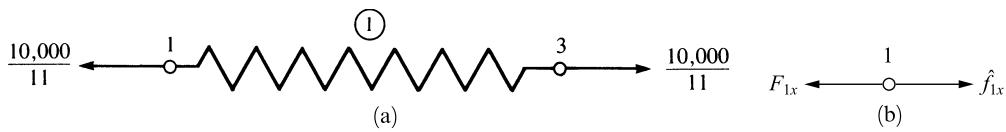(2.5.23), we obtain $$ \hat {f} _ {1 x} = \frac {- 1 0 , 0 0 0}{1 1} \mathrm{lb} \quad \hat {f} _ {3 x} = \frac {1 0 , 0 0 0}{1 1} \mathrm{lb} \tag {2.5.24} $$ A free-body diagram of spring element 1 is shown in Figure 2–10(a). The spring is subjected to tensile forces given by Eqs. (2.5.24). Also, $\hat { f } _ { 1 x }$ is equal to the reaction force $F _ { 1 x }$ given in Eq. (2.5.22). A free-body diagram of node 1 [Figure 2–10(b)] shows this result. 

text_image

10,000 11 ← 1 → 1 (a) 3 → 10,000 11 F₁ₓ ← 1 → f̂₁ₓ (b)

Figure 2–10 (a) Free-body diagram of element 1 and (b) free-body diagram of node 1. # Element 2 $$ \left\{ \begin{array}{l} \hat {f} _ {3 x} \\ \hat {f} _ {4 x} \end{array} \right\} = \left[ \begin{array}{c c} 2 0 0 0 & - 2 0 0 0 \\ - 2 0 0 0 & 2 0 0 0 \end{array} \right] \left\{ \begin{array}{l} \frac {1 0}{1 1} \\ \frac {1 5}{1 1} \end{array} \right\} \tag {2.5.25} $$ Simplifying Eq. 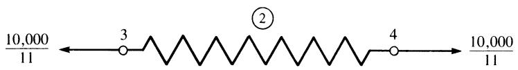(2.5.24), we obtain $$ \hat {f} _ {3 x} = \frac {- 1 0 , 0 0 0}{1 1} \mathrm{lb} \quad \hat {f} _ {4 x} = \frac {1 0 , 0 0 0}{1 1} \mathrm{lb} \tag {2.5.26} $$ A free-body diagram of spring element 2 is shown in Figure 2–11. The spring is subjected to tensile forces given by Eqs. (2.5.26). 

text_image

10,000 11 ← 3 ② 4 → 10,000 11

Figure 2–11 Free-body diagram of element 2 # Element 3 $$ \left\{ \begin{array}{l} \hat {f} _ {4 x} \\ \hat {f} _ {2 x} \end{array} \right\} = \left[ \begin{array}{c c} 3 0 0 0 & - 3 0 0 0 \\ - 3 0 0 0 & 3 0 0 0 \end{array} \right] \left\{ \begin{array}{l} \frac {1 5}{1 1} \\ 0 \end{array} \right\} \tag {2.5.27} $$ Simplifying Eq. (2.5.27) yields $$ \hat {f} _ {4 x} = \frac {4 5 , 0 0 0}{1 1} \mathrm{lb} \quad \hat {f} _ {2 x} = \frac {- 4 5 , 0 0 0}{1 1} \mathrm{lb} \tag {2.5.28} $$ 

text_image

45,000 11 → 4 → ③ → 2 → 45,000 11 (a)

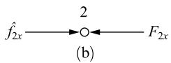
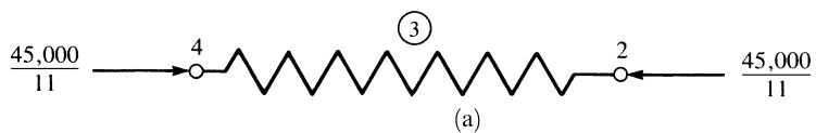
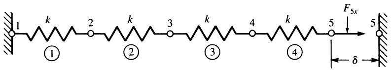
 Figure 2–12 (a) Free-body diagram of element 3 and (b) free-body diagram of node 2 A free-body diagram of spring element 3 is shown in Figure 2–12(a). The spring is subjected to compressive forces given by Eqs. (2.5.28). Also, $\hat { f } _ { 2 x }$ is equal to the reaction force $F _ { 2 x }$ given in Eq. (2.5.22). A free-body diagram of node 2 (Figure 2–12b) shows this result. # Example 2.2 For the spring assemblage shown in Figure 2–13, obtain (a) the global stiffness matrix, (b) the displacements of nodes 2–4, (c) the global nodal forces, and (d) the local element forces. Node 1 is fixed while node 5 is given a fixed, known displacement d ¼ 20:0 mm. The spring constants are all equal to $k = 2 0 0 \mathrm { k N } / \mathrm { m }$ . 

text_image

1 k 2 k 3 k 4 k 5 F_{5x} 5 ① ② ③ ④ δ

Figure 2–13 Spring assemblage for solution (a) We use Eq. (2.2.18) to express each element stiffness matrix as $$ \underline {{k}} ^ {(1)} = \underline {{k}} ^ {(2)} = \underline {{k}} ^ {(3)} = \underline {{k}} ^ {(4)} = \left[ \begin{array}{c c} 2 0 0 & - 2 0 0 \\ - 2 0 0 & 2 0 0 \end{array} \right] \tag {2.5.29} $$ Again using superposition, we obtain the global stiffness matrix as $$ \underline {{{K}}} = \left[ \begin{array}{c c c c c} 2 0 0 & - 2 0 0 & 0 & 0 & 0 \\ - 2 0 0 & 4 0 0 & - 2 0 0 & 0 & 0 \\ 0 & - 2 0 0 & 4 0 0 & - 2 0 0 & 0 \\ 0 & 0 & - 2 0 0 & 4 0 0 & - 2 0 0 \\ 0 & 0 & 0 & - 2 0 0 & 2 0 0 \end{array} \right] \frac {\mathrm{kN}}{\mathrm{m}} \tag {2.5.30} $$ (b) The global stiffness matrix, Eq. (2.5.30), relates the global forces to the global displacements as follows: $$ \left\{ \begin{array}{l} F _ {1 x} \\ F _ {2 x} \\ F _ {3 x} \\ F _ {4 x} \\ F _ {5 x} \end{array} \right\} = \left[ \begin{array}{c c c c c} 2 0 0 & - 2 0 0 & 0 & 0 & 0 \\ - 2 0 0 & 4 0 0 & - 2 0 0 & 0 & 0 \\ 0 & - 2 0 0 & 4 0 0 & - 2 0 0 & 0 \\ 0 & 0 & - 2 0 0 & 4 0 0 & - 2 0 0 \\ 0 & 0 & 0 & - 2 0 0 & 2 0 0 \end{array} \right] \left\{ \begin{array}{l} d _ {1 x} \\ d _ {2 x} \\ d _ {3 x} \\ d _ {4 x} \\ d _ {5 x} \end{array} \right\} \tag {2.5.31} $$ Applying the boundary conditions $d _ { 1 x } = 0$ and $d _ { 5 x } = 2 0$ mm $\left( = 0 . 0 2 \mathrm { m } \right)$ , substituting known global forces $F _ { 2 x } = 0 , F _ { 3 x } = 0$ , and $F _ { 4 x } = 0$ , and partitioning the first and fifth equations of Eq. (2.5.31) corresponding to these boundary conditions, we obtain $$ \left\{ \begin{array}{l} 0 \\ 0 \\ 0 \end{array} \right\} = \left[ \begin{array}{c c c c c} - 2 0 0 & 4 0 0 & - 2 0 0 & 0 & 0 \\ 0 & - 2 0 0 & 4 0 0 & - 2 0 0 & 0 \\ 0 & 0 & - 2 0 0 & 4 0 0 & - 2 0 0 \end{array} \right] \left\{ \begin{array}{c} 0 \\ d _ {2 x} \\ d _ {3 x} \\ d _ {4 x} \\ 0. 0 2 \mathrm{m} \end{array} \right\} \tag {2.5.32} $$ We now rewrite Eq. (2.5.32), transposing the product of the appropriate stiffness coefficient ð200Þ multiplied by the known displacement ð0:02 mÞ to the left side. $$ \left\{ \begin{array}{c} 0 \\ 0 \\ 4 \mathrm{kN} \end{array} \right\} = \left[ \begin{array}{c c c} 4 0 0 & - 2 0 0 & 0 \\ - 2 0 0 & 4 0 0 & - 2 0 0 \\ 0 & - 2 0 0 & 4 0 0 \end{array} \right] \left\{ \begin{array}{c} d _ {2 x} \\ d _ {3 x} \\ d _ {4 x} \end{array} \right\} \tag {2.5.33} $$ Solving Eq. (2.5.33), we obtain $$ d _ {2 x} = 0. 0 0 5 \mathrm{m} \quad d _ {3 x} = 0. 0 1 \mathrm{m} \quad d _ {4 x} = 0. 0 1 5 \mathrm{m} \tag {2.5.34} $$ (c) The global nodal forces are obtained by back-substituting the boundary condition displacements and Eqs. (2.5.34) into Eq. (2.5.31). This substitution yields $$ F _ {1 x} = (- 2 0 0) (0. 0 0 5) = - 1. 0 \mathrm{kN} $$ $$ F _ {2 x} = (4 0 0) (0. 0 0 5) - (2 0 0) (0. 0 1) = 0 $$ $$ F _ {3 x} = (- 2 0 0) (0. 0 0 5) + (4 0 0) (0. 0 1) - (2 0 0) (0. 0 1 5) = 0 \tag {2.5.35} $$ $$ F _ {4 x} = (- 2 0 0) (0. 0 1) + (4 0 0) (0. 0 1 5) - (2 0 0) (0. 0 2) = 0 $$ $$ F _ {5 x} = (- 2 0 0) (0. 0 1 5) + (2 0 0) (0. 0 2) = 1. 0 \mathrm{kN} $$ The results of Eqs. (2.5.35) yield the reaction $F _ { 1 x }$ opposite that of the nodal force $F _ { 5 x }$ required to displace node 5 by $\delta = 2 0 . 0$ mm. This result verifies equilibrium of the whole spring assemblage. (d) Next, we make use of local element Eq. (2.2.17) to obtain the forces in each element. # Element 1 $$ \left\{ \begin{array}{l} \hat {f} _ {1 x} \\ \hat {f} _ {2 x} \end{array} \right\} = \left[ \begin{array}{c c} 2 0 0 & - 2 0 0 \\ - 2 0 0 & 2 0 0 \end{array} \right] \left\{ \begin{array}{l} 0 \\ 0. 0 0 5 \end{array} \right\} \tag {2.5.36} $$ Simplifying Eq. (2.5.36) yields $$ \hat {f} _ {1 x} = - 1. 0 \mathrm{kN} \quad \hat {f} _ {2 x} = 1. 0 \mathrm{kN} \tag {2.5.37} $$ # Element 2 $$ \left\{ \begin{array}{l} \hat {f} _ {2 x} \\ \hat {f} _ {3 x} \end{array} \right\} = \left[ \begin{array}{c c} 2 0 0 & - 2 0 0 \\ - 2 0 0 & 2 0 0 \end{array} \right] \left\{ \begin{array}{l} 0. 0 0 5 \\ 0. 0 1 \end{array} \right\} \tag {2.5.38} $$ Simplifying Eq. (2.5.38) yields $$ \hat {f} _ {2 x} = - 1 \mathrm{kN} \quad \hat {f} _ {3 x} = 1 \mathrm{kN} \tag {2.5.39} $$ # Element 3 $$ \left\{ \begin{array}{l} \hat {f} _ {3 x} \\ \hat {f} _ {4 x} \end{array} \right\} = \left[ \begin{array}{c c} 2 0 0 & - 2 0 0 \\ - 2 0 0 & 2 0 0 \end{array} \right] \left\{ \begin{array}{l} 0. 0 1 \\ 0. 0 1 5 \end{array} \right\} \tag {2.5.40} $$ Simplifying Eq. (2.5.40), we have $$ \hat {f} _ {3 x} = - 1 \mathrm{kN} \quad \hat {f} _ {4 x} = 1 \mathrm{kN} \tag {2.5.41} $$ # Element 4 $$ \left\{ \begin{array}{l} \hat {f} _ {4 x} \\ \hat {f} _ {5 x} \end{array} \right\} = \left[ \begin{array}{c c} 2 0 0 & - 2 0 0 \\ - 2 0 0 & 2 0 0 \end{array} \right] \left\{ \begin{array}{l} 0. 0 1 5 \\ 0. 0 2 \end{array} \right\} \tag {2.5.42} $$ Simplifying Eq. (2.5.42), we obtain $$ \hat {f} _ {4 x} = - 1 \mathrm{kN} \quad \hat {f} _ {5 x} = 1 \mathrm{kN} \tag {2.5.43} $$ You should draw free-body diagrams of each node and element and use the results of Eqs. (2.5.35)–(2.5.43) to verify both node and element equilibria. Finally, to review the major concepts presented in this chapter, we solve the following example problem. 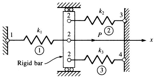# Example 2.3 (a) Using the ideas presented in Section 2.3 for the system of linear elastic springs shown in Figure 2–14, express the boundary conditions, the compatibility or continuity condition similar to Eq. (2.3.3), and the nodal equilibrium conditions similar to Eqs. (2.3.4)–(2.3.6). Then formulate the global stiffness matrix and equations for solution of the unknown global displacement and forces. The spring constants for the elements are $k _ { 1 } , k _ { 2 } .$ , and $k _ { 3 } ; P$ is an applied force at node 2. (b) Using the direct stiffness method, formulate the same global stiffness matrix and equation as in part (a). 

text_image

1 k₁ ① Rigid bar 2 2 2 k₂ 3 P② k₃ 4 3

Figure 2–14 Spring assemblage for solution (a) The boundary conditions are $$ d _ {1 x} = 0 \quad d _ {3 x} = 0 \quad d _ {4 x} = 0 \tag {2.5.44} $$ The compatibility condition at node 2 is $$ d _ {2 x} ^ {(1)} = d _ {2 x} ^ {(2)} = d _ {2 x} ^ {(3)} = d _ {2 x} \tag {2.5.45} $$ The nodal equilibrium conditions are $$ F _ {1 x} = f _ {1 x} ^ {(1)} $$ $$ P = f _ {2 x} ^ {(1)} + f _ {2 x} ^ {(2)} + f _ {2 x} ^ {(3)} \tag {2.5.46} $$ $$ F _ {3 x} = f _ {3 x} ^ {(2)} $$ $$ F _ {4 x} = f _ {4 x} ^ {(3)} $$ 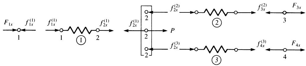where the sign convention for positive element nodal forces given by Figure 2–2 was used in writing Eqs. (2.5.46). Figure 2–15 shows the element and nodal force freebody diagrams. 

flowchart

```mermaid graph LR A["F1x"] --> B["1"] B --> C["f1x^(1)"] C --> D["1"] D --> E["f2x^(1)"] E --> F["2"] F --> G["f2x^(1)"] G --> H["2"] H --> I["P"] I --> J["f2x^(2)"] J --> K["3"] K --> L["f3x^(2)"] L --> M["3"] M --> N["F3x"] N --> O["4"] O --> P["f4x^(3)"] P --> Q["4"] ```

Figure 2–15 Free-body diagrams of elements and nodes of spring assemblage of Figure 2–14 Using the local stiffness matrix Eq. (2.2.17) applied to each element, and compatibility condition Eq. (2.5.45), we obtain the total or global equilibrium equations as $$ F _ {1 x} = k _ {1} d _ {1 x} - k _ {1} d _ {2 x} $$ $$ P = - k _ {1} d _ {1 x} + k _ {1} d _ {2 x} + k _ {2} d _ {2 x} - k _ {2} d _ {3 x} + k _ {3} d _ {2 x} - k _ {3} d _ {4 x} \tag {2.5.47} $$ $$ F _ {3 x} = - k _ {2} d _ {2 x} + k _ {2} d _ {3 x} $$ $$ F _ {4 x} = - k _ {3} d _ {2 x} + k _ {3} d _ {4 x} $$ In matrix form, we express Eqs. (2.5.47) as $$ \left\{ \begin{array}{c} F _ {1 x} \\ P \\ F _ {3 x} \\ F _ {4 x} \end{array} \right\} = \left[ \begin{array}{c c c c} k _ {1} & - k _ {1} & 0 & 0 \\ - k _ {1} & k _ {1} + k _ {2} + k _ {3} & - k _ {2} & - k _ {3} \\ 0 & - k _ {2} & k _ {2} & 0 \\ 0 & - k _ {3} & 0 & k _ {3} \end{array} \right] \left\{ \begin{array}{c} d _ {1 x} \\ d _ {2 x} \\ d _ {3 x} \\ d _ {4 x} \end{array} \right\} \tag {2.5.48} $$ Therefore, the global stiffness matrix is the square, symmetric matrix on the right side of Eq. (2.5.48). Making use of the boundary conditions, Eqs. (2.5.44), and then considering the second equation of Eqs. (2.5.47) or (2.5.48), we solve for $d _ { 2 x }$ as $$ d _ {2 x} = \frac {P}{k _ {1} + k _ {2} + k _ {3}} \tag {2.5.49} $$ We could have obtained this same result by deleting rows 1, 3, and 4 in the $\underline { { F } }$ and $\underline { d }$ matrices and rows and columns 1, 3, and 4 in $\underline { { K } } ,$ corresponding to zero displacement, as previously described in Section 2.4, and then solving for $d _ { 2 x }$ . Using Eqs. (2.5.47), we now solve for the global forces as $$ F _ {1 x} = - k _ {1} d _ {2 x} \quad F _ {3 x} = - k _ {2} d _ {2 x} \quad F _ {4 x} = - k _ {3} d _ {2 x} \tag {2.5.50} $$ The forces given by Eqs. (2.5.50) can be interpreted as the global reactions in this example. The negative signs in front of these forces indicate that they are directed to the left (opposite the x axis). (b) Using the direct stiffness method, we formulate the global stiffness matrix. First, using Eq. (2.2.18), we express each element stiffness matrix as $$ \underline {{k}} ^ {(1)} = \left[ \begin{array}{c c} d _ {1 x} & d _ {2 x} \\ k _ {1} & - k _ {1} \\ - k _ {1} & k _ {1} \end{array} \right] \underline {{k}} ^ {(2)} = \left[ \begin{array}{c c} d _ {2 x} & d _ {3 x} \\ k _ {2} & - k _ {2} \\ - k _ {2} & k _ {2} \end{array} \right] \underline {{k}} ^ {(3)} = \left[ \begin{array}{c c} d _ {2 x} & d _ {4 x} \\ k _ {3} & - k _ {3} \\ - k _ {3} & k _ {3} \end{array} \right] \tag {2.5.51} $$ where the particular degrees of freedom associated with each element are listed in the columns above each matrix. Using the direct stiffness method as outlined in Section 2.4, we add terms from each element stiffness matrix into the appropriate corresponding row and column in the global stiffness matrix to obtain $$ \underline {{{K}}} = \left[ \begin{array}{c c c c} d _ {1 x} & d _ {2 x} & d _ {3 x} & d _ {4 x} \\ k _ {1} & - k _ {1} & 0 & 0 \\ - k _ {1} & k _ {1} + k _ {2} + k _ {3} & - k _ {2} & - k _ {3} \\ 0 & - k _ {2} & k _ {2} & 0 \\ 0 & - k _ {3} & 0 & k _ {3} \end{array} \right] \tag {2.5.52} $$ We observe that each element stiffness matrix $\underline { { k } }$ has been added into the location in the global $\underline { { K } }$ corresponding to the identical degree of freedom associated with the element $\underline { { k } } .$ For instance, element 3 is associated with degrees of freedom $d _ { 2 x }$ and $d _ { 4 x }$ ; hence its contributions to $\underline { { K } }$ are in the 2–2, 2–4, 4–2, and 4–4 locations of $\underline { { K } }$ , as indicated in Eq. (2.5.52) by the $k _ { 3 }$ terms. Having assembled the global K by the direct stiffness method, we then formulate the global equations in the usual manner by making use of the general Eq. (2.3.10), $\underline { { F } } = \underline { { K } } \underline { { d } }$ . These equations have been previously obtained by Eq. (2.5.48) and therefore are not repeated. Another method for handling imposed boundary conditions that allows for either homogeneous (zero) or nonhomogeneous (nonzero) prescribed degrees of freedom is called the penalty method. This method is easy to implement in a computer program. 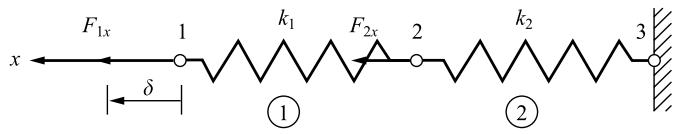Consider the simple spring assemblage in Figure 2–16 subjected to applied forces $F _ { 1 x }$ and $F _ { 2 x }$ as shown. Assume the horizontal displacement at node 1 to be forced to be $d _ { 1 x } = \delta$ . 

text_image

F_{1x} 1 k_1 F_{2x} 2 k_2 3 x ← δ ① ② 3

Figure 2–16 Spring assemblage used to illustrate the penalty method We add another spring (often called a boundary element) with a large stiffness $k _ { b }$ to the assemblage in the direction of the nodal displacement $d _ { 1 x } = \delta$ as shown in Figure $2 { - } 1 7 .$ . This spring stiffness should have a magnitude about $1 0 ^ { 6 }$ times that of the largest $k _ { i i }$ term. 

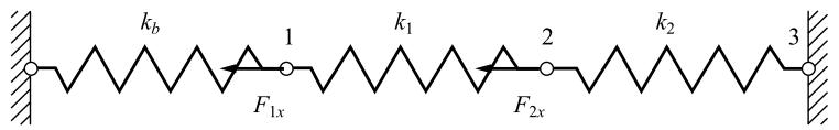
text_image

k_b 1 k_1 2 k_2 3 F_{1x} F_{2x}

Figure 2–17 Spring assemblage with a boundary spring element added at node 1 Now we add the force $k _ { b } \delta$ in the direction of $d _ { 1 x }$ and solve the problem in the usual manner as follows. The element stiffness matrices are $$ \underline {{k}} ^ {(1)} = \left[ \begin{array}{c c} k _ {1} & - k _ {1} \\ - k _ {1} & k _ {1} \end{array} \right] \quad \underline {{k}} ^ {(2)} = \left[ \begin{array}{c c} k _ {2} & - k _ {2} \\ - k _ {2} & k _ {2} \end{array} \right] \tag {2.5.53} $$ Assembling the element stiffness matrices using the direct stiffness method, we obtain the global stiffness matrix as $$ \underline {{K}} = \left[ \begin{array}{c c c} k _ {1} + k _ {b} & - k _ {1} & 0 \\ - k _ {1} & k _ {1} + k _ {2} & - k _ {2} \\ 0 & - k _ {2} & k _ {2} \end{array} \right] \tag {2.5.54} $$ Assembling the global $\underline { { F } } = \underline { { K } } \underline { { d } }$ equations and invoking the boundary condition $d _ { 3 x } = 0 .$ , we obtain $$ \left\{ \begin{array}{c} F _ {1 x} + k _ {b} \delta \\ F _ {2 x} \\ F _ {3 x} \end{array} \right\} = \left[ \begin{array}{c c c} k _ {1} + k _ {b} & - k _ {1} & 0 \\ - k _ {1} & k _ {1} + k _ {2} & - k _ {2} \\ 0 & - k _ {2} & k _ {2} \end{array} \right] \left\{ \begin{array}{c} d _ {1 x} \\ d _ {2 x} \\ d _ {3 x} = 0 \end{array} \right\} \tag {2.5.55} $$ Solving the first and second of Eqs. (2.5.55), we obtain $$ d _ {1 x} = \frac {F _ {2 x} - (k _ {1} + k _ {2}) d _ {2 x}}{- k _ {1}} \tag {2.5.56} $$ and $$ d _ {2 x} = \frac {(k _ {1} + k _ {b}) F _ {2 x} + F _ {1 x} k _ {1} + k _ {b} \delta k _ {1}}{k _ {b} k _ {1} + k _ {b} k _ {2} + k _ {1} k _ {2}} \tag {2.5.57} $$ Now as $k _ { b }$ approaches infinity, Eq. (2.5.57) simplifies to $$ d _ {2 x} = \frac {F _ {2 x} + \delta k _ {1}}{k _ {1} + k _ {2}} \tag {2.5.58} $$ and Eq. (2.5.56) simplifies to $$ d _ {1 x} = \delta \tag {2.5.59} $$ These results match those obtained by setting $d _ { 1 x } = \delta$ initially. In using the penalty method, a very large element stiffness should be parallel to a degree of freedom as is the case in the preceding example. If $k _ { b }$ were inclined, or were placed within a structure, it would contribute to both diagonal and off-diagonal coefficients in the global stiffness matrix K. This condition can lead to numerical difficulties in solving the equations F ¼ Kd. To avoid this condition, we transform the displacements at the inclined support to local ones as described in Section 3.9. # 2.6 Potential Energy Approach to Derive Spring Element Equations One of the alternative methods often used to derive the element equations and the stiffness matrix for an element is based on the principle of minimum potential energy. (The use of this principle in structural mechanics is fully described in Reference [4].) This method has the advantage of being more general than the method given in Section 2.2, which involves nodal and element equilibrium equations along with the stress/strain law for the element. Thus the principle of minimum potential energy is more adaptable to the determination of element equations for complicated elements (those with large numbers of degrees of freedom) such as the plane stress/strain element, the axisymmetric stress element, the plate bending element, and the three-dimensional solid stress element. Again, we state that the principle of virtual work (Appendix E) is applicable for any material behavior, whereas the principle of minimum potential energy is applicable only for elastic materials. However, both principles yield the same element equations for linear-elastic materials, which are the only kind considered in this text. Moreover, the principle of minimum potential energy, being included in the general category of variational methods (as is the principle of virtual work), leads to other variational functions (or functionals) similar to potential energy that can be formulated for other classes of problems, primarily of the nonstructural type. These other problems are generally classified as field problems and include, among others, torsion of a bar, heat transfer (Chapter 13), fluid flow (Chapter 14), and electric potential. Still other classes of problems, for which a variational formulation is not clearly definable, can be formulated by weighted residual methods. We will describe Galerkin’s method in Section 3.12, along with collocation, least squares, and the subdomain weighted residual methods in Section 3.13. In Section 3.13, we will also demonstrate these methods by solving a one-dimensional bar problem using each of the four residual methods and comparing each result to an exact solution. (For more information on weighted residual methods, also consult References [5–7].)