text_image

-\frac{w l}{2} ↓ 1 - \frac{w l^2}{12} ① l = 50" - \frac{w l^2}{12} ② l = 50" - \frac{w l}{2} ↓ 3 \frac{w l^2}{12} \frac{w l^2}{12}

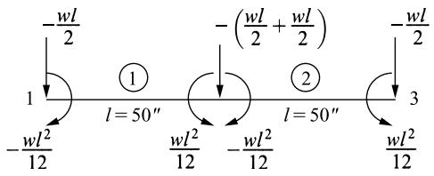
Figure 4–32 Beam discretized into two elements and work-equivalent load replacement for each element The shear force is derived by taking three derivatives on the displacement function. For the uniformly loaded beam, the resulting shear force shown in Figure 4–31(c) is a constant throughout the single-element model. Again, the best approximation for shear force is at the midpoint of the element. It should be noted that if we use Eq. (4.4.11), that is, $\underline { { f } } = \underline { { k } } \underline { { d } } - \underline { { f } } _ { o } ,$ , and subtract off the $\underline f _ { o }$ matrix, we also obtain the correct nodal forces and moments in each element. For instance, from the one-element finite element solution we have for the bending moment at node 1 $$ m _ {1} ^ {(1)} = \frac {E I}{L ^ {3}} \left[ - 6 L \left(\frac {- w L ^ {4}}{8 E I}\right) + 2 L ^ {2} \left(\frac {- w L ^ {3}}{6 E I}\right) \right] - \left(\frac {- w L ^ {2}}{1 2}\right) = \frac {w L ^ {2}}{2} $$ and at node 2 $$ m _ {2} ^ {(1)} = 0 $$ To improve the finite element solution we need to use more elements in the model (refine the mesh) or use a higher-order element, such as a fifth-order approximation for the displacement function, that is, $\hat { v } ( x ) = a _ { 1 } + a _ { 2 } x + a _ { 3 } x ^ { 2 } + a _ { 4 } x ^ { 3 } + a _ { 5 } x ^ { 4 } + a _ { 6 } x ^ { 5 }$ , with three nodes (with an extra node at the middle of the element). We now present the two-element finite element solution for the cantilever beam subjected to a uniformly distributed load. Figure 4–32 shows the beam discretized into two elements of equal length and the work-equivalent load replacement for each element. Using the beam element stiffness matrix [Eq. (4.1.13)], we obtain the element stiffness matrices as follows: $$ \underline {{k}} ^ {(1)} = \underline {{k}} ^ {(2)} = \frac {E I}{l ^ {3}} \left[ \begin{array}{c c c c} 1 & & 2 \\ 2 & & 3 \\ 1 2 & 6 l & - 1 2 & 6 l \\ 6 l & 4 l ^ {2} & - 6 l & 2 l ^ {2} \\ - 1 2 & - 6 l & 1 2 & - 6 l \\ 6 l & 2 l ^ {2} & - 6 l & 4 l ^ {2} \end{array} \right] \tag {4.5.21} $$ where l ¼ 50 in. is the length of each element and the numbers above the columns indicate the degrees of freedom associated with each element. Applying the boundary conditions $\hat { d } _ { 1 y } = 0$ and $\hat { \phi } _ { 1 } = 0$ to reduce the number of equations for a normal longhand solution, we obtain the global equations for solution as $$ \frac {E I}{l ^ {3}} \left[ \begin{array}{c c c c} 2 4 & 0 & - 1 2 & 6 l \\ 0 & 8 l ^ {2} & - 6 l & 2 l ^ {2} \\ - 1 2 & - 6 l & 1 2 & - 6 l \\ 6 l & 2 l ^ {2} & - 6 l & 4 l ^ {2} \end{array} \right] \left\{ \begin{array}{l} \hat {d} _ {2 y} \\ \hat {\phi} _ {2} \\ \hat {d} _ {3 y} \\ \hat {\phi} _ {3} \end{array} \right\} = \left\{ \begin{array}{c} - w l \\ 0 \\ - w l / 2 \\ w l ^ {2} / 1 2 \end{array} \right\} \tag {4.5.22} $$ Solving Eq. (4.5.22) for the displacements and slopes, we obtain $$ \hat {d} _ {2 y} = \frac {- 1 7 w l ^ {4}}{2 4 E I} \quad \hat {d} _ {3 y} = \frac {- 2 w l ^ {4}}{E I} \quad \hat {\phi} _ {2} = \frac {- 7 w l ^ {3}}{6 E I} \quad \hat {\phi} _ {3} = \frac {- 4 w l ^ {3}}{3 E I} \tag {4.5.23} $$ Substituting the numerical values w ¼ 20 lb/in., l ¼ 50 in., $E = 3 0 \times 1 0 ^ { 6 }$ psi, and $I = 1 0 0 \mathrm { i n . } ^ { 4 }$ into Eq. (4.5.23), we obtain $$ \hat {d} _ {2 y} = - 0. 0 2 9 5 1 \text { in. } \quad \hat {d} _ {3 y} = - 0. 0 8 3 3 \text { in. } \quad \hat {\phi} _ {2} = - 9. 7 2 2 \times 1 0 ^ {- 4} \text { rad } $$ $$ \hat {\phi} _ {3} = - 1 1. 1 1 \times 1 0 ^ {- 4} \mathrm{rad} $$ The two-element solution yields nodal displacements that match the beam theory results exactly [see Eqs. (4.5.9) and (4.5.12)]. A plot of the two-element displacement throughout the length of the beam would be a cubic displacement within each element. Within element 1, the plot would start at a displacement of 0 at node 1 and finish at a displacement of
0:0295 at node 2. A cubic function would connect these values. Similarly, within element 2, the plot would start at a displacement of
0:0295 and finish at a displacement of
0:0833 in. at node 2 [see Figure 4–31(a)]. A cubic function would again connect these values. # d 4.6 Beam Element with Nodal Hinge In some beams an internal hinge may be present. In general, this internal hinge causes a discontinuity in the slope of the deflection curve at the hinge. 

text_image

ŷ φ̂₁ ≠ 0, in general m̂₁, φ̂₁ 1 L φ̂₁y, d̂₁y φ̂₂ = 0 Hinge 2 x̂ Hi f̂₂y, d̂₂y

(a) 

text_image

eral φ̂₁ ≠ 0, in general m̂₁ = 0 Hinge L φ̂₂, m̂₂ f̂₁ᵧ, d̂₁ᵧ f̂₂ᵧ, d̂₂ᵧ

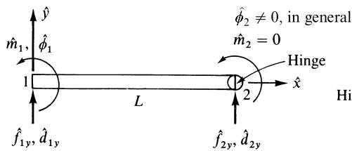
(b) Figure 4–33 Beam element with (a) hinge at right end and (b) hinge at left end Also, the bending moment is zero at the hinge. We could construct other types of connections that release other generalized end forces; that is, connections can be designed to make the shear force or axial force zero at the connection. These special conditions can be treated by starting with the generalized unreleased beam stiffness matrix [Eq. (4.1.14)] and eliminating the known zero force or moment. This yields a modified stiffness matrix with the desired force or moment equal to zero and the corresponding displacement or slope eliminated. We now consider the most common cases of a beam element with a nodal hinge at the right end or left end, as shown in Figure 4–33. For the beam element with a hinge at its right end, the moment $\hat { m } _ { 2 }$ is zero and we partition the $\underline { { \hat { k } } }$ matrix [Eq. (4.1.14)] to eliminate the degree of freedom $\hat { \phi } _ { 2 }$ (which is not zero, in general) associated with $\hat { m } _ { 2 } = 0$ as follows: $$ \underline {{\hat {k}}} = \frac {E I}{L ^ {3}} \left[ \begin{array}{c c c c} 1 2 & 6 L & - 1 2 & 6 L \\ 6 L & 4 L ^ {2} & - 6 L & 2 L ^ {2} \\ - 1 2 & - 6 L & 1 2 & - 6 L \\ \hline 6 L & 2 L ^ {2} & - 6 L & 4 L ^ {2} \end{array} \right] \tag {4.6.1} $$ We condense out the degree of freedom $\hat { \phi } _ { 2 }$ associated with $\hat { m } _ { 2 } = 0$ . Partitioning allows us to condense out the degree of freedom $\hat { \phi } _ { 2 }$ associated with $\hat { m } _ { 2 } = 0$ . That is, Eq. (4.6.1) is partitioned as shown below: $$ \hat {\underline {{k}}} = \left[ \begin{array}{c c} \underline {{K}} _ {1 1} & \underline {{K}} _ {1 2} \\ 3 \times 3 & 3 \times 1 \\ \underline {{K}} _ {2 1} & \underline {{K}} _ {2 2} \\ 1 \times 3 & 1 \times 1 \end{array} \right] \tag {4.6.2} $$ The condensed stiffness matrix is then found by using the equation $\underline { { \hat { f } } } = \underline { { \hat { k } } } \underline { { \hat { d } } }$ partitioned as follows: $$ \left\{ \begin{array}{c} \underline {{f}} _ {1} \\ 3 \times 1 \\ \underline {{f}} _ {2} \\ 1 \times 1 \end{array} \right\} = \left[ \begin{array}{c c} \underline {{K}} _ {1 1} & \underline {{K}} _ {1 2} \\ 3 \times 3 & 3 \times 1 \\ \underline {{K}} _ {2 1} & \underline {{K}} _ {2 2} \\ 1 \times 3 & 1 \times 1 \end{array} \right] \left\{ \begin{array}{c} \underline {{d}} _ {1} \\ 3 \times 1 \\ \underline {{d}} _ {2} \\ 1 \times 1 \end{array} \right\} \tag {4.6.3} $$ where $\underline { { d } } _ { 1 } = \left\{ \begin{array} { c } { \hat { d } _ { 1 y } } \\ { \hat { \phi } _ { 1 } } \\ { \hat { d } _ { 2 y } } \end{array} \right\} \qquad \underline { { d } } _ { 2 } = \{ \hat { \phi } _ { 2 } \}$ ð4:6:4Þ Equations (4.6.3) in expanded form are $$ \underline {{f}} _ {1} = \underline {{K}} _ {1 1} \underline {{d}} _ {1} + \underline {{K}} _ {1 2} \underline {{d}} _ {2} \tag {4.6.5} $$ $$ \underline {{f}} _ {2} = \underline {{K}} _ {2 1} \underline {{d}} _ {1} + \underline {{K}} _ {2 2} \underline {{d}} _ {2} $$ Solving for $\underline { { d } } _ { 2 }$ in the second of Eqs. (4.6.5), we obtain $$ \underline {{d}} _ {2} = \underline {{K}} _ {2 2} ^ {- 1} (\underline {{f}} _ {2} - \underline {{K}} _ {2 1} \underline {{d}} _ {1}) \tag {4.6.6} $$ Substituting Eq. (4.6.6) into the first of Eqs. (4.6.5), we obtain $$ \underline {{{f}}} _ {1} = (\underline {{{K}}} _ {1 1} - \underline {{{K}}} _ {1 2} \underline {{{K}}} _ {2 2} ^ {- 1} \underline {{{K}}} _ {2 1}) \underline {{{d}}} _ {1} + \underline {{{K}}} _ {1 2} \underline {{{K}}} _ {2 2} ^ {- 1} \underline {{{f}}} _ {2} \tag {4.6.7} $$ Combining the second term on the right side of Eq. (4.6.7) with $\underline { { f } } _ { 1 }$ , we obtain $$ \underline {{f}} _ {c} = \underline {{K}} _ {c} \underline {{d}} _ {1} \tag {4.6.8} $$ where the condensed stiffness matrix is $$ \underline {{K}} _ {c} = \underline {{K}} _ {1 1} - \underline {{K}} _ {1 2} \underline {{K}} _ {2 2} ^ {- 1} \underline {{K}} _ {2 1} \tag {4.6.9} $$ and the condensed force matrix is $$ \underline {{f}} _ {c} = \underline {{f}} _ {1} - \underline {{K}} _ {1 2} \underline {{K}} _ {2 2} ^ {- 1} \underline {{f}} _ {2} \tag {4.6.10} $$ Substituting the partitioned parts of $\underline { { \hat { k } } }$ from Eq. (4.6.1) into Eq. (4.6.9), we obtain the condensed stiffness matrix as $$ \begin{array}{l} \underline {{K}} _ {c} = \left[ K _ {1 1} \right] - \left[ K _ {1 2} \right] \left[ K _ {2 2} \right] ^ {- 1} \left[ K _ {2 1} \right] \\ = \frac {E I}{L ^ {3}} \left[ \begin{array}{c c c} 1 2 & 6 L & - 1 2 \\ 6 L & 4 L ^ {2} & - 6 L \\ - 1 2 & - 6 L & 1 2 \end{array} \right] - \frac {E I}{L ^ {3}} \left\{ \begin{array}{l} 6 L \\ 2 L ^ {2} \\ - 6 L \end{array} \right\} \frac {1}{4 L ^ {2}} \left[ \begin{array}{l l l} 6 L & 2 L ^ {2} & - 6 L \end{array} \right] \\ = \frac {3 E I}{L ^ {3}} \left[ \begin{array}{c c c} 1 & L & - 1 \\ L & L ^ {2} & - L \\ - 1 & - L & 1 \end{array} \right] \tag {4.6.11} \\ \end{array} $$ and the element equations (force/displacement equations) with the hinge at node 2 are $$ \left\{ \begin{array}{l} \hat {f} _ {1 y} \\ \hat {m} _ {1} \\ \hat {f} _ {2 y} \end{array} \right\} = \frac {3 E I}{L ^ {3}} \left[ \begin{array}{c c c} 1 & L & - 1 \\ L & L ^ {2} & - L \\ - 1 & - L & 1 \end{array} \right] \left\{ \begin{array}{l} \hat {d} _ {1 y} \\ \hat {\phi} _ {1} \\ \hat {d} _ {2 y} \end{array} \right\} \tag {4.6.12} $$ The generalized rotation $\hat { \phi } _ { 2 }$ has been eliminated from the equation and will not be calculated using this scheme. However, $\hat { \phi } _ { 2 }$ is not zero in general. We can expand Eq. (4.6.12) to include $\hat { \phi } _ { 2 }$ by adding zeros in the fourth row and column of the $\underline { { \hat { k } } }$ matrix to maintain $\hat { m } _ { 2 } = 0$ , as follows: $$ \left\{ \begin{array}{l} \hat {f} _ {1 y} \\ \hat {m} _ {1} \\ \hat {f} _ {2 y} \\ \hat {m} _ {2} \end{array} \right\} = \frac {3 E I}{L ^ {3}} \left[ \begin{array}{c c c c} 1 & L & - 1 & 0 \\ L & L ^ {2} & - L & 0 \\ - 1 & - L & 1 & 0 \\ 0 & 0 & 0 & 0 \end{array} \right] \left\{ \begin{array}{l} \hat {d} _ {1 y} \\ \hat {\phi} _ {1} \\ \hat {d} _ {2 y} \\ \hat {\phi} _ {2} \end{array} \right\} \tag {4.6.13} $$ For the beam element with a hinge at its left end, the moment $\hat { m } _ { 1 }$ is zero, and we partition the $\underline { { \hat { k } } }$ matrix [Eq. (4.1.14)] to eliminate the zero moment $\hat { m } _ { 1 }$ and its corresponding rotation $\hat { \phi } _ { 1 }$ to obtain $$ \left\{ \begin{array}{l} \hat {f} _ {1 y} \\ \hat {f} _ {2 y} \\ \hat {m} _ {2} \end{array} \right\} = \frac {3 E I}{L ^ {3}} \left[ \begin{array}{c c c} 1 & - 1 & L \\ - 1 & 1 & - L \\ L & - L & L ^ {2} \end{array} \right] \left\{ \begin{array}{l} \hat {d} _ {1 y} \\ \hat {d} _ {2 y} \\ \hat {\phi} _ {2} \end{array} \right\} \tag {4.6.14} $$ The expanded form of Eq. (4.6.14) including $\hat { \phi } _ { 1 }$ is $$ \left\{ \begin{array}{l} \hat {f} _ {1 y} \\ \hat {m} _ {1} \\ \hat {f} _ {2 y} \\ \hat {m} _ {2} \end{array} \right\} = \frac {3 E I}{L ^ {3}} \left[ \begin{array}{c c c c} 1 & 0 & - 1 & L \\ 0 & 0 & 0 & 0 \\ - 1 & 0 & 1 & - L \\ L & 0 & - L & L ^ {2} \end{array} \right] \left\{ \begin{array}{l} \hat {d} _ {1 y} \\ \hat {\phi} _ {1} \\ \hat {d} _ {2 y} \\ \hat {\phi} _ {2} \end{array} \right\} \tag {4.6.15} $$ # Example 4.10 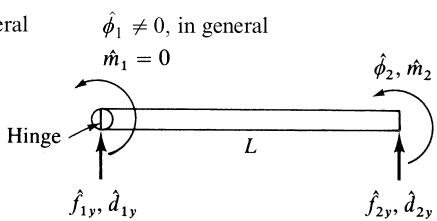Determine the displacement and rotation at node 2 and the element forces for the uniform beam with an internal hinge at node 2 shown in Figure 4–34. Let EI be a constant. 

text_image

P Hinge 1 2 2 3 a b

Figure 4–34 Beam with internal hinge We can assume the hinge is part of element 1. Therefore, using Eq. (4.6.13), the stiffness matrix of element 1 is $$ \begin{array}{c c c c} d _ {1 y} & \phi_ {1} & d _ {2 y} & \phi_ {2} \end{array} $$ $$ \underline {{k}} ^ {(1)} = \frac {3 E I}{a ^ {3}} \left[ \begin{array}{c c c c} 1 & a & - 1 & 0 \\ a & a ^ {2} & - a & 0 \\ - 1 & - a & 1 & 0 \\ 0 & 0 & 0 & 0 \end{array} \right] \tag {4.6.16} $$ The stiffness matrix of element 2 is obtained from Eq. (4.1.14) as $$ d _ {2 y} \quad \phi_ {2} \quad d _ {3 y} \quad \phi_ {3} $$ $$ \underline {{k}} ^ {(2)} = \frac {E I}{b ^ {3}} \left[ \begin{array}{c c c c} 1 2 & 6 b & - 1 2 & 6 b \\ 6 b & 4 b ^ {2} & - 6 b & 2 b ^ {2} \\ - 1 2 & - 6 b & 1 2 & - 6 b \\ 6 b & 2 b ^ {2} & - 6 b & 4 b ^ {2} \end{array} \right] \tag {4.6.17} $$ Superimposing Eqs. (4.6.16) and (4.6.17) and applying the boundary conditions $$ d _ {1 y} = 0, \quad \phi_ {1} = 0, \quad d _ {3 y} = 0, \quad \phi_ {3} = 0 $$ we obtain the total stiffness matrix and total set of equations as $$ E I \left[ \begin{array}{c c} \frac {3}{a ^ {3}} + \frac {1 2}{b ^ {3}} & \frac {6}{b ^ {2}} \\ \frac {6}{b ^ {2}} & \frac {4}{b} \end{array} \right] \left\{ \begin{array}{l} d _ {2 y} \\ \phi_ {2} \end{array} \right\} = \left\{ \begin{array}{c} - P \\ 0 \end{array} \right\} \tag {4.6.18} $$ Solving Eq. (4.6.18), we obtain $$ d _ {2 y} = \frac {- a ^ {3} b ^ {3} P}{3 \left(b ^ {3} + a ^ {3}\right) E I} \tag {4.6.19} $$ $$ \phi_ {2} = \frac {a ^ {3} b ^ {2} P}{2 (b ^ {3} + a ^ {3}) E I} $$ The value $\phi _ { 2 }$ is actually that associated with element 2—that is, $\phi _ { 2 }$ in Eq. (4.6.19) is actually $\phi _ { ? } ^ { ( 2 ) }$ . The value of $\phi _ { 2 }$ at the right end of element 1 $( \phi _ { 2 } ^ { ( 1 ) } )$ is, in general, not equal to $\phi _ { 2 } ^ { ( 2 ) }$ . If we had chosen to assume the hinge to be part of element 2, then we would have used Eq. (4.1.14) for the stiffness matrix of element 1 and Eq. (4.6.15) for the stiffness matrix of element 2. This would have enabled us to obtain $\phi _ { 2 } ^ { ( 1 ) }$ Þ, which is different from $\phi _ { 2 } ^ { ( 2 ) }$ . Using Eq. (4.6.12) for element 1, we obtain the element forces as $$ \left\{ \begin{array}{l} \hat {f} _ {1 y} \\ \hat {m} _ {1} \\ \hat {f} _ {2 y} \end{array} \right\} = \frac {3 E I}{a ^ {3}} \left[ \begin{array}{c c c} 1 & a & - 1 \\ a & a ^ {2} & - a \\ - 1 & - a & 1 \end{array} \right] \left\{ \begin{array}{c} 0 \\ 0 \\ \frac {- a ^ {3} b ^ {3} P}{3 (b ^ {3} + a ^ {3}) E I} \end{array} \right\} \tag {4.6.20} $$ Simplifying Eq. (4.6.20), we obtain the forces as $$ \hat {f} _ {1 y} = \frac {b ^ {3} P}{b ^ {3} + a ^ {3}} $$ $$ \hat {m} _ {1} = \frac {a b ^ {3} P}{b ^ {3} + a ^ {3}} \tag {4.6.21} $$ $$ \hat {f} _ {2 y} = - \frac {b ^ {3} P}{b ^ {3} + a ^ {3}} $$ Using Eq. (4.6.17) and the results from Eq. (4.6.19), we obtain the element 2 forces as $$ \left\{ \begin{array}{l} \hat {f} _ {2 y} \\ \hat {m} _ {2} \\ \hat {f} _ {3 y} \\ \hat {m} _ {3} \end{array} \right\} = \frac {E I}{b ^ {3}} \left[ \begin{array}{c c c c} 1 2 & 6 b & - 1 2 & 6 b \\ 6 b & 4 b ^ {2} & - 6 b & 2 b ^ {2} \\ - 1 2 & - 6 b & 1 2 & - 6 b \\ 6 b & 2 b ^ {2} & - 6 b & 4 b ^ {2} \end{array} \right] \left\{ \begin{array}{c} - \frac {a ^ {3} b ^ {3} P}{3 \left(b ^ {3} + a ^ {3}\right) E I} \\ \frac {a ^ {3} b ^ {2} P}{2 \left(b ^ {3} + a ^ {3}\right) E I} \\ 0 \\ 0 \end{array} \right\} \tag {4.6.22} $$ Simplifying Eq. (4.6.22), we obtain the element forces as $$ \hat {f} _ {2 y} = - \frac {a ^ {3} P}{b ^ {3} + a ^ {3}} $$ $$ \hat {m} _ {2} = 0 $$ $$ \hat {f} _ {3 y} = \frac {a ^ {3} P}{b ^ {3} + a ^ {3}} \tag {4.6.23} $$ $$ \hat {m} _ {3} = - \frac {b a ^ {3} P}{b ^ {3} + a ^ {3}} $$ It should be noted that another way to solve the nodal hinge of Example 4.10 would be to assume a nodal hinge at the right end of element one and at the left end of element two. Hence, we would use the three-equation stiffness matrix of Eq. (4.6.12) for the left element and the three-equation stiffness matrix of Eq. (4.6.14) for the right element. This results in the hinge rotation being condensed out of the global equations. You can verify that we get the same result for the displacement as given by Eq. (4.6.19). However, we must then go back to Eq. (4.6.6) using it separately for each element to obtain the rotation at node two for each element. We leave this verification to your discretion. # 4.7 Potential Energy Approach to Derive Beam Element Equations We will now derive the beam element equations using the principle of minimum potential energy. The procedure is similar to that used in Section 3.10 in deriving the bar element equations. Again, our primary purpose in applying the principle of minimum potential energy is to enhance your understanding of the principle. It will be used routinely in subsequent chapters to develop element stiffness equations. We use the same notation here as in Section 3.10. The total potential energy for a beam is $$ \pi_ {p} = U + \Omega \tag {4.7.1} $$ where the general one-dimensional expression for the strain energy U for a beam is given by $$ U = \iiint_ {V} \frac {1}{2} \sigma_ {x} \varepsilon_ {x} d V \tag {4.7.2} $$ and for a single beam element subjected to both distributed and concentrated nodal loads, the potential energy of forces is given by $$ \Omega = - \iint_ {S _ {1}} \hat {T} _ {y} \hat {v} d S - \sum_ {i = 1} ^ {2} \hat {P} _ {i y} \hat {d} _ {i y} - \sum_ {i = 1} ^ {2} \hat {m} _ {i} \hat {\phi} _ {i} \tag {4.7.3} $$ 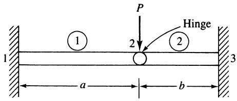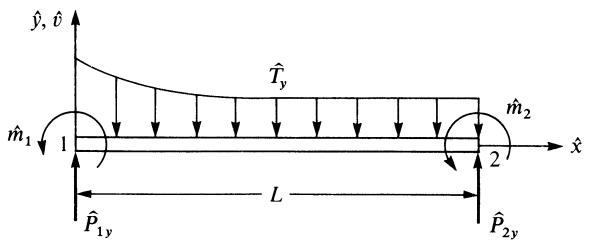where body forces are now neglected. The terms on the right-hand side of Eq. (4.7.3) represent the potential energy of (1) transverse surface loading $\hat { T } _ { y }$ (in units of force per unit surface area, acting over surface $S _ { 1 }$ and moving through displacements over which $\hat { T } _ { y }$ act); (2) nodal concentrated force $\hat { P } _ { i y }$ moving through displacements $\hat { d } _ { i y } ;$ and (3) moments $\hat { m } _ { i }$ moving through rotations $\hat { \phi _ { i } }$ . Again, v^ is the transverse displacement function for the beam element of length L shown in Figure 4–35. 

text_image

ŷ, v̂ T̂y ˆm1 1 ˆm2 2 x̂ L ˆP1y ˆP2y

Figure 4–35 Beam element subjected to surface loading and concentrated nodal forces Consider the beam element to have constant cross-sectional area A. The differential volume for the beam element can then be expressed as $$ d V = d A d \hat {x} \tag {4.7.4} $$ and the differential area over which the surface loading acts is $$ d S = b d \hat {x} \tag {4.7.5} $$ where b is the constant width. Using Eqs. (4.7.4) and (4.7.5) in Eqs. (4.7.1)–(4.7.3), the total potential energy becomes $$ \pi_ {p} = \iint_ {\hat {x}} \iint_ {A} \frac {1}{2} \sigma_ {x} \varepsilon_ {x} d A d \hat {x} - \int_ {0} ^ {L} b \hat {T} _ {y} \hat {v} d \hat {x} - \sum_ {i = 1} ^ {2} (\hat {P} _ {i y} \hat {d} _ {i y} + \hat {m} _ {i} \hat {\phi} _ {i}) \tag {4.7.6} $$ Substituting Eq. (4.1.4) for v^ into the strain/displacement relationship Eq. (4.1.10), repeated here for convenience as $$ \varepsilon_ {x} = - \hat {y} \frac {d ^ {2} \hat {v}}{d \hat {x} ^ {2}} \tag {4.7.7} $$ we express the strain in terms of nodal displacements and rotations as $$ \left\{\varepsilon_ {x} \right\} = - \hat {y} \left[ \frac {1 2 \hat {x} - 6 L}{L ^ {3}} \frac {6 \hat {x} L - 4 L ^ {2}}{L ^ {3}} \frac {- 1 2 \hat {x} + 6 L}{L ^ {3}} \frac {6 \hat {x} L - 2 L ^ {2}}{L ^ {3}} \right] \{\hat {d} \} \tag {4.7.8} $$ or $\{ \varepsilon _ { x } \} = - \hat { y } [ B ] \{ \hat { d } \}$ ð4:7:9Þ where we define $$ [ B ] = \left[ \frac {1 2 \hat {x} - 6 L}{L ^ {3}} \frac {6 \hat {x} L - 4 L ^ {2}}{L ^ {3}} \frac {- 1 2 \hat {x} + 6 L}{L ^ {3}} \frac {6 \hat {x} L - 2 L ^ {2}}{L ^ {3}} \right] \tag {4.7.10} $$ The stress/strain relationship is given by $$ \{\sigma_ {x} \} = [ D ] \{\varepsilon_ {x} \} \tag {4.7.11} $$ where $[ D ] = [ E ]$ ð4:7:12Þ and E is the modulus of elasticity. Using Eq. (4.7.9) in Eq. (4.7.11), we obtain $$ \{\sigma_ {x} \} = - \hat {y} [ D ] [ B ] \{\hat {d} \} \tag {4.7.13} $$ Next, the total potential energy Eq. (4.7.6) is expressed in matrix notation as $$ \pi_ {p} = \iint_ {\hat {x}} \iint_ {A} \frac {1}{2} \left\{\sigma_ {x} \right\} ^ {T} \left\{\varepsilon_ {x} \right\} d A d \hat {x} - \int_ {0} ^ {L} b \hat {T} _ {y} [ \hat {v} ] ^ {T} d \hat {x} - \left\{\hat {d} \right\} ^ {T} \left\{\hat {P} \right\} \tag {4.7.14} $$ Using Eqs. (4.1.5), (4.7.9), (4.7.12), and (4.7.13), and defining $w = b \hat { T } _ { \nu }$ as the line load (load per unit length) in the y^ direction, we express the total potential energy, Eq. (4.7.14), in matrix form as $$ \pi_ {p} = \int_ {0} ^ {L} \frac {E I}{2} \{\hat {d} \} ^ {T} [ B ] ^ {T} [ B ] \{\hat {d} \} d \hat {x} - \int_ {0} ^ {L} w \{\hat {d} \} ^ {T} [ N ] ^ {T} d \hat {x} - \{\hat {d} \} ^ {T} \{\hat {P} \} \tag {4.7.15} $$ where we have used the definition of the moment of inertia $$ I = \iint_ {A} y ^ {2} d A \tag {4.7.16} $$ to obtain the first term on the right-hand side of Eq. (4.7.15). In Eq. (4.7.15), $\pi _ { p }$ is now expressed as a function of $\{ \hat { d } \}$ . Differentiating $\pi _ { p }$ in Eq. (4.7.15) with respect to $\hat { d } _ { 1 y } , \hat { \phi } _ { 1 } , \hat { d } _ { 2 y }$ , and $\hat { \phi } _ { 2 }$ and equating each term to zero to minimize $\pi _ { p } .$ , we obtain four element equations, which are written in matrix form as $$ E I \int_ {0} ^ {L} [ B ] ^ {T} [ B ] d \hat {x} \{\hat {d} \} - \int_ {0} ^ {L} [ N ] ^ {T} w d \hat {x} - \{\hat {P} \} = 0 \tag {4.7.17} $$ The derivation of the four element equations is left as an exercise (see Problem 4.45). Representing the nodal force matrix as the sum of those nodal forces resulting from distributed loading and concentrated loading, we have $$ \{\hat {f} \} = \int_ {0} ^ {L} [ N ] ^ {T} w d \hat {x} + \{\hat {P} \} \tag {4.7.18} $$ Using Eq. (4.7.18), the four element equations given by explicitly evaluating Eq. (4.7.17) are then identical to Eq. (4.1.13). The integral term on the right side of Eq. (4.7.18) also represents the work-equivalent replacement of a distributed load by nodal concentrated loads. For instance, letting $w ( \hat { x } ) = - w$ (constant), substituting shape functions from Eq. (4.1.7) into the integral, and then performing the integration result in the same nodal equivalent loads as given by Eqs. (4.4.5)–(4.4.7). Because $\{ \hat { f } \} = [ \hat { k } ] \{ \hat { d } \}$ , we have, from Eq. (4.7.17), $$ [ \hat {k} ] = E I \int_ {0} ^ {L} [ B ] ^ {T} [ B ] d \hat {x} \tag {4.7.19} $$ Using Eq. (4.7.10) in Eq. (4.7.19) and integrating, $[ \hat { k } ]$ is evaluated in explicit form as $$ [ \hat {k} ] = \frac {E I}{L ^ {3}} \left[ \begin{array}{c c c c} 1 2 & 6 L & - 1 2 & 6 L \\ & 4 L ^ {2} & - 6 L & 2 L ^ {2} \\ & & 1 2 & - 6 L \\ \text { Symmetry } & & & 4 L ^ {2} \end{array} \right] \tag {4.7.20} $$ Equation (4.7.20) represents the local stiffness matrix for a beam element. As expected, Eq. (4.7.20) is identical to Eq. (4.1.14) developed previously. # 4.8 Galerkin’s Method for Deriving Beam Element Equations We will now illustrate Galerkin’s method to formulate the beam element stiffness equations. We begin with the basic differential Eq. (4.1.1h) with transverse loading w now included; that is, $$ E I \frac {d ^ {4} \hat {v}}{d \hat {x} ^ {4}} + w = 0 \tag {4.8.1} $$ We now define the residual R to be Eq. (4.8.1). Applying Galerkin’s criterion [Eq. (3.12.3)] to Eq. (4.8.1), we have $$ \int_ {0} ^ {L} \left(E I \frac {d ^ {4} \hat {v}}{d \hat {x} ^ {4}} + w\right) N _ {i} d \hat {x} = 0 \quad (i = 1, 2, 3, 4) \tag {4.8.2} $$ where the shape functions $N _ { i }$ are defined by Eqs. (4.1.7). We now apply integration by parts twice to the first term in Eq. (4.8.2) to yield $$ \int_ {0} ^ {L} E I (\hat {v}, _ {\hat {x} \hat {x} \hat {x} \hat {x}}) N _ {i} d \hat {x} = \int_ {0} ^ {L} E I (\hat {v}, _ {\hat {x} \hat {x}}) (N _ {i}, _ {\hat {x} \hat {x}}) d \hat {x} + E I [ N _ {i} (\hat {v}, _ {\hat {x} \hat {x} \hat {x}}) - (N _ {i}, _ {\hat {x}}) (\hat {v}, _ {\hat {x} \hat {x}}) ] _ {0} ^ {L} \tag {4.8.3} $$ where the notation of the comma followed by the subscript x^ indicates differentiation with respect to x^. Again, integration by parts introduces the boundary conditions. Because $\hat { v } = [ N ] \{ \hat { d } \}$ as given by Eq. (4.1.5), we have $$ \hat {v} _ {, \hat {x} \hat {x}} = \left[ \frac {1 2 \hat {x} - 6 L}{L ^ {3}} \frac {6 \hat {x} L - 4 L ^ {2}}{L ^ {3}} \frac {- 1 2 \hat {x} + 6 L}{L ^ {3}} \frac {6 \hat {x} L - 2 L ^ {2}}{L ^ {3}} \right] \{\hat {d} \} \tag {4.8.4} $$ or, using Eq. (4.7.10), $$ \hat {v}, _ {\hat {x} \hat {x}} = [ B ] \{\hat {d} \} \tag {4.8.5} $$ Substituting Eq. (4.8.5) into Eq. (4.8.3), and then Eq. (4.8.3) into Eq. (4.8.2), we obtain $$ \int_ {0} ^ {L} (N _ {i, \hat {x} \hat {x}}) E I [ B ] d \hat {x} \{\hat {d} \} + \int_ {0} ^ {L} N _ {i} w d \hat {x} + [ N _ {i} \hat {V} - (N _ {i, \hat {x}}) \hat {m} ] | _ {0} ^ {L} = 0 \quad (i = 1, 2, 3, 4) \tag {4.8.6} $$ where Eqs. (4.1.11) have been used in the boundary terms. Equation (4.8.6) is really four equations (one each for $N _ { i } = N _ { 1 } , N _ { 2 } , N _ { 3 }$ , and $N _ { 4 } )$ . Instead of directly evaluating Eq. (4.8.6) for each $N _ { i } ,$ , as was done in Section 3.12, we can express the four equations of Eq. (4.8.6) in matrix form as $$ \int_ {0} ^ {L} [ B ] ^ {T} E I [ B ] d \hat {x} \{\hat {d} \} = \int_ {0} ^ {L} - [ N ] ^ {T} w d \hat {x} + ([ N ] ^ {T}, _ {\hat {x}} \hat {m} - [ N ] ^ {T} \hat {V}) | _ {0} ^ {L} \tag {4.8.7} $$ where we have used the relationship $[ N ] , _ { x x } = [ B ]$ in Eq. (4.8.7). Observe that the integral term on the left side of Eq. (4.8.7) is identical to the stiffness matrix previously given by Eq. (4.7.19) and that the first term on the right side of Eq. (4.8.7) represents the equivalent nodal forces due to distributed loading [also given in Eq. (4.7.18)]. The two terms in parentheses on the right side of Eq. (4.8.7) are the same as the concentrated force matrix $\{ \hat { P } \}$ of Eq. (4.7.18). We explain this by evaluating $[ N ] , _ { \hat { x } }$ and ½N, where ½N is defined by Eq. (4.1.6), at the ends of the element as follows: $$ \left[ N \right] _ {, \hat {x}} \mid_ {0} = \left[ \begin{array}{l l l l} 0 & 1 & 0 & 0 \end{array} \right] \quad \left[ N \right] _ {, \hat {x}} \mid_ {L} = \left[ \begin{array}{l l l l} 0 & 0 & 0 & 1 \end{array} \right] \tag {4.8.8} $$ $$ [ N ] | _ {0} = [ 1 \quad 0 \quad 0 \quad 0 ] \qquad [ N ] | _ {L} = [ 0 \quad 0 \quad 1 \quad 0 ] $$ Therefore, when we use Eqs. (4.8.8) in Eq. (4.8.7), the following terms result: $$ \left\{ \begin{array}{l} 0 \\ 0 \\ 0 \\ 1 \end{array} \right\} \hat {m} (L) - \left\{ \begin{array}{l} 0 \\ 1 \\ 0 \\ 0 \end{array} \right\} \hat {m} (0) - \left\{ \begin{array}{l} 0 \\ 0 \\ 1 \\ 0 \end{array} \right\} \hat {V} (L) + \left\{ \begin{array}{l} 1 \\ 0 \\ 0 \\ 0 \end{array} \right\} \hat {V} (0) \tag {4.8.9} $$ These nodal shear forces and moments are illustrated in Figure 4–36.