6.22. The four-node plane strain finite element shown carries at time $t$ the second Piola-Kirchhoff stresses $$ \delta \mathbf {S} = \left[ \begin{array}{c c c} 1 0 0 & 5 0 & 0 \\ 5 0 & 2 0 0 & 0 \\ 0 & 0 & 1 0 0 \end{array} \right] $$ The deformation gradient at time $t$ is $$ \mathbf {\delta} _ {6} ^ {t} \mathbf {X} = \left[ \begin{array}{l l l} 2 & 1 & 0 \\ 0 & 2 & 0 \\ 0 & 0 & 1 \end{array} \right] $$ 

text_image

x2 2 1 Time 0 0V 3 4 x1 1

(a) Sketch the deformed configuration at time t. (b) A rigid body rotation of 30 degrees counterclockwise is applied from time t to time $t + \Delta t$ to the element. Sketch the configuration at time $t + \Delta t$ . (c) Calculate corresponding to the stationary Cartesian coordinate system (i) the Cauchy stresses at time t, (ii) the Cauchy stresses at time $t + \Delta t$ , and (iii) the second Piola-Kirchhoff stresses at time $t + \Delta t$ . 6.23. The second Piola-Kirchhoff stresses $\delta S$ are for the plane strain four-node element as shown. (a) Calculate the Cauchy stresses at time t. (b) Obtain the second Piola-Kirchhoff stresses at time $t + \Delta t$ , $t^{+}\Delta t$ , S, and the Cauchy stresses at time $t + \Delta t$ , $t^{+}\Delta t$ . All stress components are measured in the stationary coordinate system $x_{1}$ , $x_{2}$ . 

text_image

Unit thickness at all times Rotated by 45° from time t to time t + Δt x2 x1 2 Configuration at time t 2 × 2 square at time 0 x1 1 3 45° 3 1 2 Unit thickness at all times Configuration at time t x1 x2 t₀S₁₁ = 40 t₀S₂₂ = -60 t₀S₃₃ = -15 t₀S₁₂ = t₀S₂₃ = t₀S₃₁ = 0

6.24. We have used a computer program to perform the following finite element analysis. 

text_image

R ① Large displacements, large strains, plane strain analysis x₂ x₁

We would like to verify that the program is working properly. As part of this verification, we consider the displacements of element 1: 

flowchart

```mermaid graph TD A["1"] -->|s| B["2"] B -->|1.5| C["3"] C -->|45°| D["4"] D -->|1| E["1"] style A fill:#f9f,stroke:#333 style B fill:#f9f,stroke:#333 style C fill:#f9f,stroke:#333 style D fill:#f9f,stroke:#333 style E fill:#f9f,stroke:#333 ```


text_image

s 2 1 2 r 3 2 4 Time t

(a) Calculate the $2 \times 2$ deformation gradient $\mathbf{t}_{0}\mathbf{X}$ at the centroid of the element. (Hint: Remember that $\mathbf{t}_{0}\mathbf{X} = \mathbf{t}_{t}\mathbf{X}^{-1}$ .) (b) The program also prints out the Cauchy stresses at the centroid of the element: $$ \left[ \begin{array}{l} ^ {t} \tau_ {1 1} \\ ^ {t} \tau_ {2 2} \\ ^ {t} \tau_ {1 2} \end{array} \right] = \left[ \begin{array}{l} 2 0. 5 0 \\ 2 0. 5 0 \\ 1 2. 5 0 \end{array} \right] $$ The material law used in the analysis is given by $$ \left[ \begin{array}{l} _ {0} ^ {t} S _ {1 1} \\ _ {0} ^ {t} S _ {2 2} \\ _ {0} ^ {t} S _ {1 2} \end{array} \right] = \left[ \begin{array}{c c c} 1 1 & 7 & 0 \\ 7 & 1 1 & 0 \\ 0 & 0 & 9 \end{array} \right] \left[ \begin{array}{l} _ {0} ^ {t} \epsilon_ {1 1} \\ _ {0} ^ {t} \epsilon_ {2 2} \\ _ {0} ^ {t} \epsilon_ {1 2} \end{array} \right] $$ Show that the Cauchy stresses printed by the program are not correct and compute the correct Cauchy stresses based on the given element displacements. Can you identify the program error? # 6.25. Consider the sheet of material shown. Here $$ ^ \prime u _ {1} = - \frac {1}{2} ^ {0} x _ {1} + 3; \quad^ {\prime} u _ {2} = \frac {1}{2} ^ {0} x _ {2} + 2. 5 $$ Also, the stresses are $$ ^ t \tau_ {1 1} = - 1 0 \mathrm{psi} $$ $$ ^ \prime \tau_ {2 2} = 2 0 \mathrm{psi} $$ $$ ^ \prime \tau_ {1 2} = 0 $$ Identify six simple independent virtual displacement patterns and show that the principle of virtual work is satisfied for these patterns. 

text_image

tfx2 = 20 psi (tension) Thickness = 1 in tfx1 = 10 psi (compression) Configuration at time t 1 in x1 2 in Configuration at time 0 2 in x2

# 6.26. Consider the one-dimensional large strain analysis of the bar shown. 

text_image

0A 0x fB 0L

$f^{B}$ = body force per unit original volume $^{0}A$ = cross-sectional area at time 0 Truss material is incompressible (a) For a cross section of the bar, derive an expression for the second Piola-Kirchhoff stress as a function of the Cauchy stress, the area ratio $^{1}A/^{0}A$ , and the deformation gradient. (b) Starting from the principle of virtual work, derive the governing differential equation of equilibrium in terms of quantities referred to the original configuration. Also, derive the boundary conditions. (c) Now rewrite the governing differential equation in terms of quantities referred to the current configuration and compare this equation with the differential equation associated with small strain analysis. 6.27. Consider a thin disk spinning around its symmetry axis with constant angular velocity $\omega$ as shown. The disk is subjected to large displacements. Specialize the general equations of the principle of virtual work in Tables 6.2 and 6.3 to this case. In the analysis, only the displacements of the disk particles in the $x_{1}$ direction are considered. 

text_image

A ω A


text_image

Section AA x2 b a H H, h << b 0V x1 h

6.28. Consider the four-node plane strain element shown. The nodal point displacements at time $t$ and time $t + \Delta t$ are shown. Calculate the incremental Green-Lagrange strain tensor components $_0\epsilon$ from time $t$ to time $t + \Delta t$ . 

text_image

x2 1 4 At time t + Δt At time t At time 0 (original configuration) 4 1 2 4 x1

6.29. In the derivations in Section 6.2.3 we used $$ \int_ {0 _ {V}} ^ {t + \Delta_ {0} ^ {t}} S _ {i j} \delta^ {t + \Delta_ {0} ^ {t}} \epsilon_ {i j} d ^ {0} V = \int_ {0 _ {V}} ^ {t + \Delta_ {0} ^ {t}} S _ {i j} \delta_ {0} \epsilon_ {i j} d ^ {0} V $$ and hence, here $\delta_{0}^{\prime}\epsilon_{ij}=0$ . But we also used $$ \int_ {0 _ {V}} \delta_ {0} S _ {i j} \delta_ {0} e _ {i j} d ^ {0} V = \int_ {0 _ {V}} \delta_ {0} S _ {i j} \delta_ {0} \epsilon_ {i j} d ^ {0} V $$ and hence, here $\delta_{0}e_{ij} = \delta_{0}'\epsilon_{ij}$ and clearly $\delta_{0}'\epsilon_{ij} \neq 0$ . Discuss briefly why all these equations are correct. 6.30. Establish the second Piola-Kirchhoff stresses ${}_{0}^{t}S_{ij}$ and the variations in the Green-Lagrange strains $\delta_0^t\epsilon_{ij}$ for the disk in Exercise 6.27 and show explicitly that for this case, $\int_{t_V}{}^t\tau_{ij}\delta_1e_{ij}d^t V = \int_{0_V}{}^t S_{ij}\delta_0^t\epsilon_{ij}d^0 V$ is indeed true. # 6.3 DISPLACEMENT-BASED ISOPARAMETRIC CONTINUUM FINITE ELEMENTS In the previous section we developed the linearized principle of virtual displacements (linearized about the state at time t) in continuum form. The only variables in the equations are the displacements of the material particles. If finite elements with only nodal point displacements as degrees of freedom are considered, then the governing finite element matrices corresponding to a full linearization of the principle of virtual displacements about the state at time t can be obtained directly by use of the equations given in the previous section. The key point to note is that in this case the element degrees of freedom, i.e., the element displacements, are exactly the variables with respect to which the general principle of virtual displacements has been linearized. Let us consider the following derivation to emphasize this point. This derivation will also show that if other than displacement degrees of freedom are used, such as rotations in structural elements or stresses in mixed formulations, the linearization with respect to such finite element degrees of freedom is more efficiently achieved by a direct Taylor series expansion with respect to such variables. # 6.3.1 Linearization of the Principle of Virtual Work with Respect to Finite Element Variables The principle of virtual displacements in the total Lagrangian formulation is given by $$ \int_ {0 _ {V}} ^ {t + \Delta t} S _ {i j} \delta^ {t + \Delta t} \epsilon_ {i j} d ^ {0} V = ^ {t + \Delta t} \mathcal {R} \tag {6.89} $$ Let us linearize this expression with respect to a general finite element nodal degree of freedom $a_k$ , where $a_k$ may be a displacement or rotation. We assume that $t + \Delta t \mathcal{R}$ is independent of the deformations. We then have, using a Taylor series expansion, $$ { } ^ { t + \Delta t } { } _ { 0 } S _ { i j } \delta ^ { t + \Delta t } { } _ { 0 } \epsilon _ { i j } \doteq { } _ { 0 } ^ { t } S _ { i j } \delta _ { 0 } ^ { t } \epsilon _ { i j } + \frac { \partial } { \partial ^ { t } a _ { k } } \left( { } _ { 0 } ^ { t } S _ { i j } \delta _ { 0 } ^ { t } \epsilon _ { i j } \right) d a _ { k } \tag {6.90} $$ where $da_{k}$ is a differential increment in $a_{k}$ . We note that $$ \delta_ {0} ^ {l} \epsilon_ {i j} = \frac {\partial_ {0} ^ {l} \epsilon_ {i j}}{\partial^ {l} a _ {l}} \delta a _ {l} \tag {6.91} $$ where $\delta a_{l}$ is a variation in $'a_{l}$ , and hence the variation is taken with respect to the nodal parameter $'a_{l}$ about the configuration at time t. The second term in (6.90) may be chain-differentiated to obtain $$ \begin{array}{l} \frac {\partial}{\partial^ {t} a _ {k}} \left(_ {0} ^ {t} S _ {i j} \delta_ {0} ^ {t} \epsilon_ {i j}\right) d a _ {k} = \frac {\partial_ {0} ^ {t} S _ {i j}}{\partial^ {t} a _ {k}} \delta_ {0} ^ {t} \epsilon_ {i j} d a _ {k} + _ {0} ^ {t} S _ {i j} \frac {\partial}{\partial^ {t} a _ {k}} \left(\delta_ {0} ^ {t} \epsilon_ {i j}\right) d a _ {k} \\ = \left(\frac {\partial_ {0} ^ {l} S _ {i j}}{\partial_ {0} ^ {l} \epsilon_ {r s}} \frac {\partial_ {0} ^ {l} \epsilon_ {r s}}{\partial^ {l} a _ {k}}\right) \left(\frac {\partial_ {0} ^ {l} \epsilon_ {i j}}{\partial^ {l} a _ {l}} \delta a _ {l}\right) d a _ {k} + \delta S _ {i j} \frac {\partial}{\partial^ {l} a _ {k}} \left(\frac {\partial_ {0} ^ {l} \epsilon_ {i j}}{\partial^ {l} a _ {l}} \delta a _ {l}\right) d a _ {k} \tag {6.92} \\ = _ {0} C _ {i j r s} \frac {\partial_ {0} ^ {t} \epsilon_ {r s}}{\partial^ {t} a _ {k}} \frac {\partial_ {0} ^ {t} \epsilon_ {i j}}{\partial^ {t} a _ {l}} \delta a _ {l} d a _ {k} + _ {0} ^ {t} S _ {i j} \frac {\partial^ {2} {} _ {0} ^ {t} \epsilon_ {i j}}{\partial^ {t} a _ {k} \partial^ {t} a _ {l}} \delta a _ {l} d a _ {k} \\ \end{array} $$ where in the last step we used $$ \frac {\partial_ {0} ^ {t} S _ {i j}}{\partial_ {0} ^ {t} \epsilon_ {r s}} = _ {0} C _ {i j r s} \tag {6.93} $$ Using the definition of the Green-Lagrange strain, we further have $$ \frac {\partial_ {0} ^ {t} \epsilon_ {i j}}{\partial^ {t} a _ {k}} = \frac {1}{2} \left(\frac {\partial_ {0} ^ {t} u _ {i , j}}{\partial^ {t} a _ {k}} + \frac {\partial_ {0} ^ {t} u _ {j , i}}{\partial^ {t} a _ {k}} + \dot {0} u _ {m, i} \frac {\partial_ {0} ^ {t} u _ {m , j}}{\partial^ {t} a _ {k}} + \dot {0} u _ {m, j} \frac {\partial_ {0} ^ {t} u _ {m , i}}{\partial^ {t} a _ {k}}\right) \tag {6.94} $$ and $\frac{\partial^2\mathbf{\Phi}_0^\prime\epsilon_{ij}}{\partial^\prime a_k\partial^\prime a_l} = \frac{1}{2}\left(\mathbf{\Phi}_0x_{m,i}\frac{\partial^2\mathbf{\Phi}_0^\prime u_{m,j}}{\partial^\prime a_k\partial^\prime a_l} +\mathbf{\Phi}_0x_{m,j}\frac{\partial^2\mathbf{\Phi}_0^\prime u_{m,i}}{\partial^\prime a_k\partial^\prime a_l} +\frac{\partial_0^\prime u_{m,i}}{\partial^\prime a_k}\frac{\partial_0^\prime u_{m,j}}{\partial^\prime a_l} +\frac{\partial_0^\prime u_{m,i}}{\partial^\prime a_l}\frac{\partial_0^\prime u_{m,j}}{\partial^\prime a_k}\right)$ (6.95) The substitution of (6.90) and (6.92) into the principle of virtual displacements (6.89) gives $$ \left\{\int C _ {i j r s} \frac {\partial_ {0} ^ {t} \epsilon_ {r s}}{\partial^ {t} a _ {k}} \frac {\partial_ {0} ^ {t} \epsilon_ {i j}}{\partial^ {t} a _ {l}} d ^ {0} V + \int S _ {i j} \frac {\partial^ {2} {} _ {0} ^ {t} \epsilon_ {i j}}{\partial^ {t} a _ {k} \partial^ {t} a _ {l}} d ^ {0} V \right\} d a _ {k} \delta a _ {l} = ^ {t + \Delta t} \mathcal {R} _ {l} - \left(\int S _ {i j} \frac {\partial_ {0} ^ {t} \epsilon_ {i j}}{\partial^ {t} a _ {l}} d ^ {0} V\right) \delta a _ {l} \tag {6.96} $$ where ${}^{t+\Delta t}R_{l}$ denotes the external virtual work corresponding to $\delta a_{l}$ . If we now compare the expression in (6.96) [and using (6.94) and (6.95)] with the linearized principle of virtual displacement expression in Table 6.2, we recognize that for isoparametric displacement-based continuum elements with nodal displacement degrees of freedom only, both expressions can directly, and easily, be employed to obtain the same finite element equations. However, for elements with rotational degrees of freedom, the expression in (6.96) may be more direct for the derivation of the fully linearized finite element equations. Namely, the second derivatives of the displacement gradients with respect to the nodal point variables appearing in (6.95) are then not zero, and their effect also needs to be included. Consequently, if the continuum linearizations in Tables 6.2 and 6.3 are used, it must be recognized that the terms ${}_{0}^{t}S_{ij}\delta_{0}e_{ij}$ and ${}^{t}\tau_{ij}\delta_{t}e_{ij}$ , on the right-hand side of the equations, still contribute terms to the stiffness matrix when ${}_{0}e_{ij}$ and ${}_{t}e_{ij}$ are not a linear function of the nodal point variables (see Section 6.5). If, in addition, other than displacement and rotational element degrees of freedom are used, then certainly the above approach of linearization is very effective (see Section 6.4 for the derivation of the displacement/pressure formulations). Here we have considered only a total Lagrangian formulation but should recognize that the same procedure of linearization is also applicable to updated Lagrangian formulations, and to all these formulations with all different material descriptions. The same procedure can also be employed to linearize the external virtual work term in (6.89) in case the loading is deformation dependent. # 6.3.2 General Matrix Equations of Displacement-Based Continuum Elements Let us now consider in more detail the matrices of isoparametric continuum finite elements with displacement degrees of freedom only. The basic steps in the derivation of the governing finite element equations are the same as those used in linear analysis: the selection of the interpolation functions and the interpolation of the element coordinates and displacements with these functions in the governing continuum mechanics equations. By invoking the linearized principle of virtual displacements for each of the nodal point displacements in turn, the governing finite element equations are obtained. As in linear analysis, we need to consider only a single element of a specific type in this derivation because the governing equilibrium equations of an assemblage of elements can be constructed using the direct stiffness procedure. In considering the element coordinate and displacement interpolations, we should recognize that it is important to employ the same interpolations for the coordinates and displacements at any and all times during the motion of the element. Since the new element coordinates are obtained by adding the element displacements to the original coordinates, it follows that the use of the same interpolations for the displacements and coordinates represents a consistent solution approach, and means that the discussions on convergence requirements in Sections 4.3 and 5.3.3 are directly applicable to the incremental analysis. In particular, it is then ensured that an assemblage of elements that are displacement-compatible across element boundaries in the original configuration will preserve this compatibility in all subsequent configurations. In Sections 6.2.3 and 6.3.1 we derived the basic incremental equations used in our finite element formulations. While in practice an iteration is necessary, we also recognized that the equations in Tables 6.2 and 6.3 and Section 6.3.1 are the basic relations that are used in such iterations. Hence, in the following presentation we only need to focus on the basic incremental equations derived in Tables 6.2 and 6.3 (with the discussion in Section 6.3.1) and summarized in (6.74) and (6.75). Substituting now the element coordinate and displacement interpolations into these equations as we did in linear analysis, we obtain—for a single element or for an assemblage of elements— in materially-nonlinear-only analysis: static analysis: $$ ^ \prime \mathbf {K} \mathbf {U} = ^ {\prime + \Delta} {} ^ {\prime} \mathbf {R} - ^ {\prime} \mathbf {F} \tag {6.97} $$ dynamic analysis, implicit time integration: $$ \mathbf {M} ^ {\prime + \Delta t} \ddot {\mathbf {U}} + ^ {t} \mathbf {K} \mathbf {U} = ^ {t + \Delta t} \mathbf {R} - ^ {t} \mathbf {F} \tag {6.98} $$ dynamic analysis, explicit time integration: $$ \mathbf {M} ^ {\prime} \ddot {\mathbf {U}} = ^ {\prime} \mathbf {R} - ^ {\prime} \mathbf {F} \tag {6.99} $$ using the TL formulation: static analysis: $$ \left(_ {0} ^ {t} \mathbf {K} _ {L} + _ {0} ^ {t} \mathbf {K} _ {N L}\right) \mathbf {U} = ^ {t + \Delta t} \mathbf {R} - _ {0} ^ {t} \mathbf {F} \tag {6.100} $$ dynamic analysis, implicit time integration: $$ \mathbf {M} ^ {t + \Delta t} \ddot {\mathbf {U}} + \left(_ {0} ^ {t} \mathbf {K} _ {L} + _ {0} ^ {t} \mathbf {K} _ {N L}\right) \mathbf {U} = ^ {t + \Delta t} \mathbf {R} - _ {0} ^ {t} \mathbf {F} \tag {6.101} $$ dynamic analysis, explicit time integration: $$ \mathbf {M} ^ {\prime} \ddot {\mathbf {U}} = ^ {\prime} \mathbf {R} - _ {0} ^ {\prime} \mathbf {F} \tag {6.102} $$ and using the UL formulation: static analysis: $$ \left(_ {t} ^ {t} \mathbf {K} _ {L} + _ {t} ^ {t} \mathbf {K} _ {N L}\right) \mathbf {U} = ^ {t + \Delta t} \mathbf {R} - _ {t} ^ {t} \mathbf {F} \tag {6.103} $$ dynamic analysis, implicit time integration: $$ \mathbf {M} ^ {t + \Delta t} \ddot {\mathbf {U}} + \left(_ {t} ^ {t} \mathbf {K} _ {L} + _ {t} ^ {t} \mathbf {K} _ {N L}\right) \mathbf {U} = ^ {t + \Delta t} \mathbf {R} - _ {t} ^ {t} \mathbf {F} \tag {6.104} $$ dynamic analysis, explicit time integration: $$ \mathbf {M} ^ {\prime} \ddot {\mathbf {U}} = ^ {\prime} \mathbf {R} - ^ {\prime} \mathbf {F} \tag {6.105} $$ where $\mathbf{M} =$ time-independent mass matrix $^{1}$ K = linear strain incremental stiffness matrix, not including the initial displacement effect $\delta\mathbf{K}_{L},\delta\mathbf{K}_{L}=linear strain incremental stiffness matrices$ $\delta\mathbf{K}_{NL},\;^{\prime}\mathbf{K}_{NL}=nonlinear strain (geometric or initial stress) incremental stiffness matrices$ $^{t+\Delta t}R = \text{vector of externally applied nodal point loads at time } t + \Delta t; \text{ this vector is also used at time } t \text{ in explicit time integration}$ $^{'}F, ^{'}F, ^{'}F = vectors of nodal point forces equivalent to the element stresses at time t$ $\mathbf{U} =$ vector of increments in the nodal point displacements $^{t}\ddot{\mathbf{U}}, ^{t+\Delta t}\ddot{\mathbf{U}} = \text{vectors of nodal point accelerations at times } t \text{ and } t + \Delta t$ In the above finite element discretization we have assumed that damping effects are negligible or can be modeled in the nonlinear constitutive relationships (for example, by use of a strain-rate-dependent material law). We also assumed that the externally applied loads are deformation-independent, and thus the load vector corresponding to all load (or time) steps can be calculated prior to the incremental analysis. If the loads include deformation-dependent components, it is necessary to update and iterate on the load vector as briefly discussed in Section 6.2.3. The above finite element matrices are evaluated as in linear analysis. Table 6.4 summarizes—for a single element—the basic integrals being considered and the corresponding matrix evaluations. The following notation is used for the calculation of the element matrices: $H^{S}, H = surface- and volume-displacement interpolation matrices$ $^{t+\Delta_{0}}\mathbf{f}^{S}, ^{t+\Delta_{0}}\mathbf{f}^{B}=$ vectors of surface and body forces defined per unit area and per unit volume of the element at time 0 $B_{L}, \mathbf{\Phi}_{0}^{t}B_{L}, \mathbf{\Phi}^{t}B_{L} = \text{linear strain-displacement transformation matrices}; B_{L} \text{ is equal to } \mathbf{\Phi}_{0}^{t}B_{L} \text{ when the initial displacement effect is neglected}$ $^{t}$ B $_{NL}$ , $^{t}$ B $_{NL}$ = nonlinear strain-displacement transformation matrices C = stress-strain material property matrix (incremental or total) $_{0}$ C, $_{t}$ C = incremental stress-strain material property matrices $^{'}\tau, ^{'}\hat{\tau} = \text{matrix and vector of Cauchy stresses}$ $\delta S, \hat{S} = \text{matrix and vector of second Piola-Kirchhoff stresses}$ $\dot{\Sigma} = \text{vector of stresses in materially-nonlinear-only analysis}$ TABLE 6.4 Finite element matrices

Analysis type	Integral	Matrix evaluation
In all analyses	$\int_{0_V}^{0} \rho^{t+\Delta t} \ddot{u}_i \delta u_i d^0 V$ $^{t+\Delta t} \mathcal{R} = \int_{0_{S_f}}^{t+\Delta t} f_i^S \delta u_i^S d^0 S$ $+ \int_{0_V}^{t+\Delta t} f_i^B \delta u_i d^0 V$	$\mathbf{M}^{t+\Delta t} \hat{\mathbf{u}} = \left( \int_{0_V}^{0} \rho \mathbf{H}^T \mathbf{H} d^0 V \right)^{t+\Delta t} \hat{\mathbf{u}}$ $^{t+\Delta t} \mathbf{R} = \int_{0_{S_f}} \mathbf{H}^{S^T}^{t+\Delta t} \mathbf{f}^S d^0 S$ $+ \int_{0_V} \mathbf{H}^{T}^{t+\Delta t} \mathbf{f}^B d^0 V$
Materially-nonlinear-only	$\int_V C_{ijrs} e_{rs} \delta e_{ij} dV$ $\int_V ^t \sigma_{ij} \delta e_{ij} dV$	$^t \mathbf{K} \hat{\mathbf{u}} = \left( \int_V \mathbf{B}^T \mathbf{C} \mathbf{B}_L dV \right) \hat{\mathbf{u}}$ $^t \mathbf{F} = \int_V \mathbf{B}^T ^t \hat{\mathbf{\Sigma}} dV$
Total Lagrangian formulation	$\int_{0_V}^{0} C_{ijrs} e_{rs} \delta_0 e_{ij} d^0 V$ $\int_{0_V}^{0} S_{ij} \delta_0 \eta_{ij} d^0 V$ $\int_{0_V}^{0} S_{ij} \delta_0 e_{ij} d^0 V$	$^0 \mathbf{K}_L \hat{\mathbf{u}} = \left( \int_{0_V} ^0 \mathbf{B}^T _0 \mathbf{C} ^0 \mathbf{B}_L d^0 V \right) \hat{\mathbf{u}}$ $^0 \mathbf{K}_{NL} \hat{\mathbf{u}} = \left( \int_{0_V} ^0 \mathbf{B}^T _NL ^0 \mathbf{S} ^0 \mathbf{B}_{NL} d^0 V \right) \hat{\mathbf{u}}$ $^0 \mathbf{F} = \int_{0_V} ^0 \mathbf{B}^T _0 \hat{\mathbf{S}} d^0 V$
Updated Lagrangian formulation	$\int_{t_V} ^t C_{ijrs} e_{rs} \delta_t e_{ij} d^t V$ $\int_{t_V} ^t \tau_{ij} \delta_t \eta_{ij} d^t V$ $\int_{t_V} ^t \tau_{ij} \delta_t e_{ij} d^t V$	$^t \mathbf{K}_L \hat{\mathbf{u}} \left( \int_{t_V} ^t \mathbf{B}^T _t \mathbf{C} ^t \mathbf{B}_L d^t V \right) \hat{\mathbf{u}}$ $^t \mathbf{K}_{NL} \hat{\mathbf{u}} = \left( \int_{t_V} ^t \mathbf{B}^T _NL ^t \tau ^t \mathbf{B}_{NL} d^t V \right) \hat{\mathbf{u}}$ $^t \mathbf{F} = \int_{t_V} ^t \mathbf{B}^T _t ^t \hat{\mathbf{r}} d^t V$

These matrices depend on the specific element considered. The displacement interpolation matrices are simply assembled as in linear analysis from the displacement interpolation functions. In the following sections we discuss the calculation of the strain-displacement and stress matrices and vectors pertaining to the continuum elements that we considered earlier for linear analysis in Chapter 5. The discussion is abbreviated because the basic numerical procedures employed in the calculation of the nonlinear finite matrices are those that we have already covered. For example, we consider again variable-number-nodes elements whose interpolation functions were previously given. As before, the displacement interpolations and strain-displacement matrices are expressed in terms of the isoparametric coordinates. Thus, the integrations indicated in Table 6.4 are performed as explained in Section 5.5. In the following discussion we consider only the UL and TL formulations because the matrices of the materially-nonlinear-only analysis can be directly obtained from these formulations, and we are only concerned with the required kinematic expressions. The evaluation of the stresses and stress-strain matrices of the elements depends on the material model used. These considerations are discussed in Section 6.6. # 6.3.3 Truss and Cable Elements As discussed previously in Section 4.2.3, a truss element is a structural member capable of transmitting stresses only in the direction normal to the cross section. It is assumed that this normal stress is constant over the cross-sectional area. 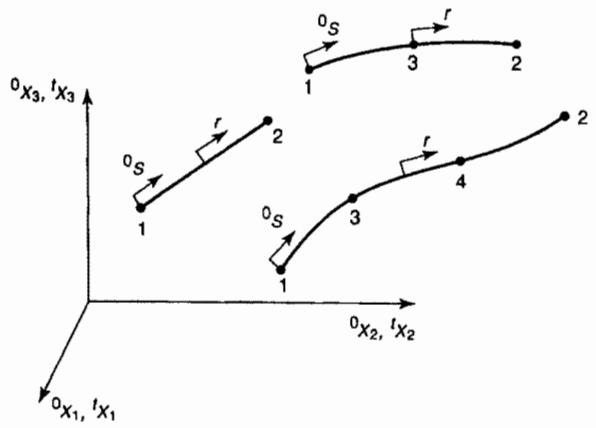In the following we consider a truss element that has an arbitrary orientation in space. The element is described by two to four nodes, as shown in Fig. 6.3, and is subjected to large displacements and large strains. The global coordinates of the nodal points of the element are at time 0, $^0 x_1^k$ , $^0 x_2^k$ , $^0 x_3^k$ and at time $t$ , $'x_1^k$ , $'x_2^k$ , $'x_3^k$ , where $k = 1, \ldots, N$ , with $N$ equal to the number of nodes ( $2 \leq N \leq 4$ ). These nodal point coordinates are assumed to determine the spatial configuration of the truss at time 0 and time $t$ using $$ { } ^ { 0 } x _ { 1 } ( r ) = \sum _ { k = 1 } ^ { N } h _ { k } { } ^ { 0 } x _ { 1 } ^ { k } ; \quad { } ^ { 0 } x _ { 2 } ( r ) = \sum _ { k = 1 } ^ { N } h _ { k } { } ^ { 0 } x _ { 2 } ^ { k } ; \quad { } ^ { 0 } x _ { 3 } ( r ) = \sum _ { k = 1 } ^ { N } h _ { k } { } ^ { 0 } x _ { 3 } ^ { k } \tag {6.106} $$ and $^{t}x_{1}(r) = \sum_{k=1}^{N} h_{k} ^{t} x_{1}^{k};$ $^{t}x_{2}(r) = \sum_{k=1}^{N} h_{k} ^{t} x_{2}^{k};$ $^{t}x_{3}(r) = \sum_{k=1}^{N} h_{k} ^{t} x_{3}^{k}$ (6.107) where the interpolation functions $h_k(r)$ have been defined in Fig. 5.3. Using (6.106) and (6.107), it follows that $$ { } ^ { t } u _ { i } ( r ) = \sum _ { k = 1 } ^ { N } h _ { k } { } ^ { t } u _ { i } ^ { k } \tag {6.108} $$ and $u_{i}(r) = \sum_{k = 1}^{N}h_{k}u_{i}^{k},\qquad i = 1,2,3$ (6.109) 

text_image

0x3, tx3 0S 1 r 2 0S 1 0x2, tx2 0x1, tx1 0S 3 r 4 2

Figure 6.3 Two- to four-node truss element Since for the truss element the only stress is the normal stress on its cross-sectional area, we consider only the corresponding longitudinal strain. Denoting the local element longitudinal strain by a curl, we have in the TL formulation, $$ \tilde {\epsilon} _ {1 1} = \frac {d ^ {0} x _ {i}}{d ^ {0} s} \frac {d ^ {t} u _ {i}}{d ^ {0} s} + \frac {1}{2} \frac {d ^ {t} u _ {i}}{d ^ {0} s} \frac {d ^ {t} u _ {i}}{d ^ {0} s} \tag {6.110} $$