where, from Eq. (5.4.16), the local stiffness matrix for a grid element is $$ \hat {\underline {{k}}} _ {G} = \left[ \begin{array}{c c c c c c} \hat {d} _ {1 y} & \hat {\phi} _ {1 x} & \hat {\phi} _ {1 z} & \hat {d} _ {2 y} & \hat {\phi} _ {2 x} & \hat {\phi} _ {2 z} \\ \frac {1 2 E I}{L ^ {3}} & 0 & \frac {6 E I}{L ^ {2}} & \frac {- 1 2 E I}{L ^ {3}} & 0 & \frac {6 E I}{L ^ {2}} \\ 0 & \frac {G J}{L} & 0 & 0 & \frac {- G J}{L} & 0 \\ \frac {6 E I}{L ^ {2}} & 0 & \frac {4 E I}{L} & \frac {- 6 E I}{L ^ {2}} & 0 & \frac {2 E I}{L} \\ \frac {- 1 2 E I}{L ^ {3}} & 0 & \frac {- 6 E I}{L ^ {2}} & \frac {1 2 E I}{L ^ {3}} & 0 & \frac {- 6 E I}{L ^ {2}} \\ 0 & \frac {- G J}{L} & 0 & 0 & \frac {G J}{L} & 0 \\ \frac {6 E I}{L ^ {2}} & 0 & \frac {2 E I}{L} & \frac {- 6 E I}{L ^ {2}} & 0 & \frac {4 E I}{L} \end{array} \right] \tag {5.4.17} $$ and the degrees of freedom are in the order (1) vertical deflection, (2) torsional rotation, and (3) bending rotation, as indicated by the notation used above the columns of Eq. (5.4.17). 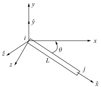The transformation matrix relating local to global degrees of freedom for a grid is given by $$ \underline {{{T}}} _ {G} = \left[ \begin{array}{c c c c c c} 1 & 0 & 0 & 0 & 0 & 0 \\ 0 & C & S & 0 & 0 & 0 \\ 0 & - S & C & 0 & 0 & 0 \\ 0 & 0 & 0 & 1 & 0 & 0 \\ 0 & 0 & 0 & 0 & C & S \\ 0 & 0 & 0 & 0 & - S & C \end{array} \right] \tag {5.4.18} $$ where y is now positive, taken counterclockwise from x to x^ in the x-z plane (Figure 5–17) and $$ C = \cos \theta = \frac {x _ {j} - x _ {i}}{L} \quad S = \sin \theta = \frac {z _ {j} - z _ {i}}{L} $$ 

text_image

y ŷ i x θ z L j x̂

Figure 5–17 Grid element arbitrarily oriented in the x-z plane where L is the length of the element from node i to node j. As indicated by Eq. (5.4.18) for a grid, the vertical deflection $\hat { d } _ { y }$ is invariant with respect to a coordinate transformation (that is, y ¼ y^) (Figure 5–17). The global stiffness matrix for a grid element arbitrarily oriented in the x-z plane is then given by using Eqs. (5.4.17) and (5.4.18) in $$ \underline {{k}} _ {G} = \underline {{T}} _ {G} ^ {T} \hat {\underline {{k}}} _ {G} \underline {{T}} _ {G} \tag {5.4.19} $$ Now that we have formulated the global stiffness matrix for the grid element, the procedure for solution then follows in the same manner as that for the plane frame. To illustrate the use of the equations developed in Section 5.4, we will now solve the following grid structures. 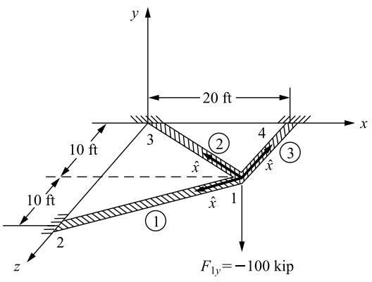# Example 5.5 Analyze the grid shown in Figure 5–18. The grid consists of three elements, is fixed at nodes 2, 3, and 4, and is subjected to a downward vertical force (perpendicular to the x-z plane passing through the grid elements) of 100 kip. The global-coordinate axes have been established at node 3, and the element lengths are shown in the figure. Let $E = 3 0 \times 1 0 ^ { 3 }$ ksi, $G = 1 2 \times 1 0 ^ { 3 }$ ksi, $I = 4 0 0 ~ \mathrm { i n } ^ { 4 }$ , and $J = 1 1 0 \mathrm { i n } ^ { 4 }$ for all elements of the grid. 

text_image

y 20 ft x 10 ft 3 ② 4 x̂ ③ 10 ft x̂ 1 ① 2 z F₁y = -100 kip

Figure 5–18 Grid for analysis showing local x^ axis for each element Substituting Eq. (5.4.17) for the local stiffness matrix and Eq. (5.4.18) for the transformation matrix into Eq. (5.4.19), we can obtain each element global stiffness matrix. To expedite the longhand solution, the boundary conditions at nodes 2, 3, and 4, $$ d _ {2 y} = \phi_ {2 x} = \phi_ {2 z} = 0 \quad d _ {3 y} = \phi_ {3 x} = \phi_ {3 z} = 0 \quad d _ {4 y} = \phi_ {4 x} = \phi_ {4 z} = 0 \tag {5.4.20} $$ make it possible to use only the upper left-hand 3  3 partitioned part of the local stiffness and transformation matrices associated with the degrees of freedom at node 1. Therefore, the global stiffness matrices for each element are as follows: # Element 1 For element 1, we assume the local x^ axis to be directed from node 1 to node 2 for the formulation of the element stiffness matrix. We need the following expressions to evaluate the element stiffness matrix: $$ \begin{array}{l} C = \cos \theta = \frac {x _ {2} - x _ {1}}{L ^ {(1)}} = \frac {- 2 0 - 0}{2 2 . 3 6} = - 0. 8 9 4 \\ S = \sin \theta = \frac {z _ {2} - z _ {1}}{L ^ {(1)}} = \frac {1 0 - 0}{2 2 . 3 6} = 0. 4 4 7 \\ \frac {1 2 E I}{L ^ {3}} = \frac {1 2 (3 0 \times 1 0 ^ {3}) (4 0 0)}{(2 2 . 3 6 \times 1 2) ^ {3}} = 7. 4 5 \tag {5.4.21} \\ \frac {6 E I}{L ^ {2}} = \frac {6 (3 0 \times 1 0 ^ {3}) (4 0 0)}{(2 2 . 3 6 \times 1 2) ^ {2}} = 1 0 0 0 \\ \frac {G J}{L} = \frac {(1 2 \times 1 0 ^ {3}) (1 1 0)}{(2 2 . 3 6 \times 1 2)} = 4 9 2 0 \\ \frac {4 E I}{L} = \frac {4 (3 0 \times 1 0 ^ {3}) (4 0 0)}{(2 2 . 3 6 \times 1 2)} = 1 7 9, 0 0 0 \\ \end{array} $$ Considering the boundary condition Eqs. (5.4.20), using the results of Eqs. (5.4.21) in Eq. (5.4.17) for $\underline { { \hat { k } } } _ { G }$ and Eq. (5.4.18) for $\underline { { T } } _ { G } .$ , and then applying Eq. (5.4.19), we obtain the upper left-hand $3 \times 3$ partitioned part of the global stiffness matrix for element 1 as $$ \underline {{k}} ^ {(1)} = \left[ \begin{array}{c c c} 1 & 0 & 0 \\ 0 & - 0. 8 9 4 & - 0. 4 4 7 \\ 0 & 0. 4 4 7 & - 0. 8 9 4 \end{array} \right] \left[ \begin{array}{c c c} 7. 4 5 & 0 & 1 0 0 0 \\ 0 & 4 9 2 0 & 0 \\ 1 0 0 0 & 0 & 1 7 9, 0 0 0 \end{array} \right] \left[ \begin{array}{c c c} 1 & 0 & 0 \\ 0 & - 0. 8 9 4 & 0. 4 4 7 \\ 0 & - 0. 4 4 7 & - 0. 8 9 4 \end{array} \right] $$ Performing the matrix multiplications, we obtain the global element grid stiffness matrix $$ \underline {{k}} ^ {(1)} = \left[ \begin{array}{c c c} d _ {1 y} & \phi_ {1} & \phi_ {2} \\ 7. 4 5 & - 4 4 7 & - 8 9 4 \\ - 4 4 7 & 3 9, 7 0 0 & 6 9, 6 0 0 \\ - 8 9 4 & 6 9, 6 0 0 & 1 4 4, 0 0 0 \end{array} \right] \frac {\mathrm{kip}}{\text { in. }} \tag {5.4.22} $$ where the labels next to the columns indicate the degrees of freedom. # Element 2 For element 2, we assume the local x^ axis to be directed from node 1 to node 3 for the formulation of the element stiffness matrix. We need the following expressions to evaluate the element stiffness matrix: $$ C = \frac {x _ {3} - x _ {1}}{L ^ {(2)}} = \frac {- 2 0 - 0}{2 2 . 3 6} = - 0. 8 9 4 \tag {5.4.23} $$ $$ S = \frac {z _ {3} - z _ {1}}{L ^ {(2)}} = \frac {- 1 0 - 0}{2 2 . 3 6} = - 0. 4 4 7 $$ Other expressions used in Eq. (5.4.17) are identical to those in Eqs. (5.4.21) for element 1 because E; G; I; J, and L are identical. Evaluating Eq. (5.4.19) for the global stiffness matrix for element 2, we obtain $$ \underline {{k}} ^ {(2)} = \left[ \begin{array}{c c c} 1 & 0 & 0 \\ 0 & - 0. 8 9 4 & 0. 4 4 7 \\ 0 & - 0. 4 4 7 & - 0. 8 9 4 \end{array} \right] \left[ \begin{array}{c c c} 7. 4 5 & 0 & 1 0 0 0 \\ 0 & 4 9 2 0 & 0 \\ 1 0 0 0 & 0 & 1 7 9, 0 0 0 \end{array} \right] \left[ \begin{array}{c c c} 1 & 0 & 0 \\ 0 & - 0. 8 9 4 & - 0. 4 4 7 \\ 0 & 0. 4 4 7 & - 0. 8 9 4 \end{array} \right] $$ Simplifying, we obtain $$ \underline {{k}} ^ {(2)} = \left[ \begin{array}{c c c} d _ {1 y} & \phi_ {1 x} & \phi_ {1 z} \\ 7. 4 5 & 4 4 7 & - 8 9 4 \\ 4 4 7 & 3 9, 7 0 0 & - 6 9, 6 0 0 \\ - 8 9 4 & - 6 9, 6 0 0 & 1 4 4, 0 0 0 \end{array} \right] \frac {\mathrm{kip}}{\mathrm{in.}} \tag {5.4.24} $$ # Element 3 For element 3, we assume the local x^ axis to be directed from node 1 to node 4. We need the following expressions to evaluate the element stiffness matrix: $$ \begin{array}{l} C = \frac {x _ {4} - x _ {1}}{L ^ {(3)}} = \frac {2 0 - 2 0}{1 0} = 0 \\ S = \frac {z _ {4} - z _ {1}}{L ^ {(3)}} = \frac {0 - 1 0}{1 0} = - 1 \tag {5.4.25} \\ \frac {1 2 E I}{L ^ {3}} = \frac {1 2 (3 0 \times 1 0 ^ {3}) (4 0 0)}{(1 0 \times 1 2) ^ {3}} = 8 3. 3 \\ \frac {6 E I}{L ^ {2}} = \frac {6 (3 0 \times 1 0 ^ {3}) (4 0 0)}{(1 0 \times 1 2) ^ {2}} = 5 0 0 0 \\ \end{array} $$ $$ \frac {G J}{L} = \frac {(1 2 \times 1 0 ^ {3}) (1 1 0)}{(1 0 \times 1 2)} = 1 1, 0 0 0 $$ $$ \frac {4 E I}{L} = \frac {4 (3 0 \times 1 0 ^ {3}) (4 0 0)}{(1 0 \times 1 2)} = 4 0 0, 0 0 0 $$ Using Eqs. (5.4.25), we can obtain the upper part of the global stiffness matrix for element 3 as $$ \underline {{{{k}}}} ^ {(3)} = \left[ \begin{array}{c c c} d _ {1 y} & \phi_ {1 x} & \phi_ {1 z} \\ 8 3. 3 & 5 0 0 0 & 0 \\ 5 0 0 0 & 4 0 0, 0 0 0 & 0 \\ 0 & 0 & 1 1, 0 0 0 \end{array} \right] \frac {\mathrm{kip}}{\text {in.}} \tag {5.4.26} $$ Superimposing the global stiffness matrices from Eqs. (5.4.22), (5.4.24), and (5.4.26), we obtain the total stiffness matrix of the grid (with boundary conditions applied) as $$ \underline {{{K}}} _ {G} = \left[ \begin{array}{c c c} d _ {1 y} & \phi_ {1 x} & \phi_ {1 z} \\ 9 8. 2 & 5 0 0 0 & - 1 7 9 0 \\ 5 0 0 0 & 4 7 9, 0 0 0 & 0 \\ - 1 7 9 0 & 0 & 2 9 9, 0 0 0 \end{array} \right] \frac {\mathrm{kip}}{\text {in.}} \tag {5.4.27} $$ The grid matrix equation then becomes $$ \left\{ \begin{array}{l} F _ {1 y} = - 1 0 0 \\ M _ {1 x} = 0 \\ M _ {1 z} = 0 \end{array} \right\} = \left[ \begin{array}{c c c} 9 8. 2 & 5 0 0 0 & - 1 7 9 0 \\ 5 0 0 0 & 4 7 9, 0 0 0 & 0 \\ - 1 7 9 0 & 0 & 2 9 9, 0 0 0 \end{array} \right] \left\{ \begin{array}{l} d _ {1 y} \\ \phi_ {1 x} \\ \phi_ {1 z} \end{array} \right\} \tag {5.4.28} $$ The force $F _ { 1 y }$ is negative because the load is applied in the negative y direction. Solving for the displacement and the rotations in Eq. (5.4.28), we obtain $$ d _ {1 y} = - 2. 8 3 \text { in. } $$ $$ \phi_ {1 x} = 0. 0 2 9 5 \mathrm{rad} \tag {5.4.29} $$ $$ \phi_ {1 z} = - 0. 0 1 6 9 \mathrm{rad} $$ The results indicate that the y displacement at node 1 is downward as indicated by the minus sign, the rotation about the x axis is positive, and the rotation about the z axis is negative. Based on the downward loading location with respect to the supports, these results are expected. Having solved for the unknown displacement and the rotations, we can obtain the local element forces on formulating the element equations in a manner similar to that for the beam and the plane frame. The local forces (which are needed in the design/analysis stage) are found by applying the equation $\underline { { \hat { f } } } = \underline { { \hat { k } } } _ { G } \underline { { T } } _ { G } \underline { { d } }$ for each element as follows: # Element 1 Using Eqs. (5.4.17) and (5.4.18) for $\underline { { \hat { k } } } _ { G }$ and $\underline { { T } } _ { G }$ and Eq. (5.4.29), we obtain $$ \underline {{T}} _ {G} \underline {{d}} = \left[ \begin{array}{c c c c c c} 1 & 0 & 0 & 0 & 0 & 0 \\ 0 & - 0. 8 9 4 & 0. 4 4 7 & 0 & 0 & 0 \\ 0 & - 0. 4 4 7 & - 0. 8 9 4 & 0 & 0 & 0 \\ 0 & 0 & 0 & 1 & 0 & 0 \\ 0 & 0 & 0 & 0 & - 0. 8 9 4 & 0. 4 4 7 \\ 0 & 0 & 0 & 0 & - 0. 4 4 7 & - 0. 8 9 4 \end{array} \right] \left\{ \begin{array}{c} - 2. 8 3 \\ 0. 0 2 9 5 \\ - 0. 0 1 6 9 \\ 0 \\ 0 \\ 0 \end{array} \right\} $$ Multiplying the matrices, we obtain $$ \underline {{T}} _ {G} \underline {{d}} = \left\{ \begin{array}{c} - 2. 8 3 \\ - 0. 0 3 3 9 \\ 0. 0 0 1 9 2 \\ 0 \\ 0 \\ 0 \end{array} \right\} \tag {5.4.30} $$ Then $\underline { { \hat { f } } } = \underline { { \hat { k } } } _ { G } \underline { { T } } _ { G } \underline { { d } }$ becomes $$ \left\{ \begin{array}{l} \hat {f} _ {1 y} \\ \hat {m} _ {1 x} \\ \hat {m} _ {1 z} \\ \hat {f} _ {2 y} \\ \hat {m} _ {2 x} \\ \hat {m} _ {2 z} \end{array} \right\} = \left[ \begin{array}{c c c c c c} 7. 4 5 & 0 & 1 0 0 0 & - 7. 4 5 & 0 & 1 0 0 0 \\ 0 & 4 9 2 0 & 0 & 0 & - 4 9 2 0 & 0 \\ 1 0 0 0 & 0 & 1 7 9, 0 0 0 & - 1 0 0 0 & 0 & 8 9, 5 0 0 \\ - 7. 4 5 & 0 & - 1 0 0 0 & 7. 4 5 & 0 & - 1 0 0 0 \\ 0 & - 4 9 2 0 & 0 & 0 & 4 9 2 0 & 0 \\ 1 0 0 0 & 0 & 8 9, 5 0 0 & - 1 0 0 0 & 0 & 1 7 9, 0 0 0 \end{array} \right] \left\{ \begin{array}{l} - 2. 8 3 \\ - 0. 0 3 3 9 \\ 0. 0 0 1 9 2 \\ 0 \\ 0 \\ 0 \end{array} \right\} \tag {5.4.31} $$ Multiplying the matrices in Eq. (5.4.31), we obtain the local element forces as $$ \left\{ \begin{array}{l} \hat {f} _ {1 y} \\ \hat {m} _ {1 x} \\ \hat {m} _ {1 z} \\ \hat {f} _ {2 y} \\ \hat {m} _ {2 x} \\ \hat {m} _ {2 z} \end{array} \right\} = \left\{ \begin{array}{c} - 1 9. 2 \text { kip } \\ - 1 6 7 \text { k - in. } \\ - 2 4 8 0 \text { k - in. } \\ 1 9. 2 \text { kip } \\ 1 6 7 \text { k - in. } \\ - 2 6 6 0 \text { k - in. 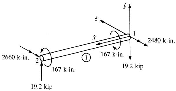} \end{array} \right\} \tag {5.4.32} $$ The directions of the forces acting on element 1 are shown in the free-body diagram of element 1 in Figure 5–19.  

text_image

2660 k-in. 2 167 k-in. 19.2 kip 1 167 k-in. 19.2 kip 2480 k-in. 1 x ŷ z x̂ ①

Figure 5–19 Free-body diagrams of the elements of Figure 5–18 showing local-coordinate systems for each # Element 2 Similarly, using $\underline { { \hat { f } } } = \underline { { \hat { k } } } _ { G } \underline { { T } } _ { G } \underline { { d } }$ for element 2, with the direction cosines in Eqs. (5.4.23), we obtain $$ \left\{ \begin{array}{l} \hat {f} _ {1 y} \\ \hat {m} _ {1 x} \\ \hat {m} _ {1 z} \\ \hat {f} _ {3 y} \\ \hat {m} _ {3 x} \\ \hat {m} _ {3 z} \end{array} \right\} = \left[ \begin{array}{c c c c c c} 7. 4 5 & 0 & 1 0 0 0 & - 7. 4 5 & 0 & 1 0 0 0 \\ 0 & 4 9 2 0 & 0 & 0 & - 4 9 2 0 & 0 \\ 1 0 0 0 & 0 & 1 7 9, 0 0 0 & - 1 0 0 0 & 0 & 8 9, 5 0 0 \\ - 7. 4 5 & 0 & - 1 0 0 0 & 7. 4 5 & 0 & - 1 0 0 0 \\ 0 & - 4 9 2 0 & 0 & 0 & 4 9 2 0 & 0 \\ 1 0 0 0 & 0 & 8 9, 5 0 0 & - 1 0 0 0 & 0 & 1 7 9, 0 0 0 \end{array} \right] $$ $$ \times \left[ \begin{array}{c c c c c c} 1 & 0 & 0 & 0 & 0 & 0 \\ 0 & - 0. 8 9 4 & - 0. 4 4 7 & 0 & 0 & 0 \\ 0 & 0. 4 4 7 & - 0. 8 9 4 & 0 & 0 & 0 \\ 0 & 0 & 0 & 1 & 0 & 0 \\ 0 & 0 & 0 & 0 & - 0. 8 9 4 & - 0. 4 4 7 \\ 0 & 0 & 0 & 0 & 0. 4 4 7 & - 0. 8 9 4 \end{array} \right] \left\{ \begin{array}{c} - 2. 8 3 \\ 0. 0 2 9 5 \\ - 0. 0 1 6 9 \\ 0 \\ 0 \\ 0 \end{array} \right\} \tag {5.4.33} $$ Multiplying the matrices in Eq. (5.4.33), we obtain the local element forces as $$ \hat {f} _ {1 y} = 7. 2 3 \mathrm{kip} $$ $$ \hat {m} _ {1 x} = - 9 2. 5 \mathrm{k-in}. $$ $$ \hat {m} _ {1 z} = 2 2 4 0 \mathrm{k} - \text {in}. \tag {5.4.34} $$ $$ \hat {f} _ {3 y} = - 7. 2 3 \mathrm{kip} $$ $$ \hat {m} _ {3 x} = 9 2. 5 \mathrm{k-in}. $$ $$ \hat {m} _ {3 z} = - 2 9 5 \mathrm{k} \text {-in}. $$ # Element 3 Finally, using the direction cosines in Eqs. (5.4.25), we obtain the local element forces as $$ \left\{ \begin{array}{l} \hat {f} _ {1 y} \\ \hat {m} _ {1 x} \\ \hat {m} _ {1 z} \\ \hat {f} _ {3 y} \\ \hat {m} _ {3 x} \\ \hat {m} _ {3 z} \end{array} \right\} = \left[ \begin{array}{c c c c c c} 8 3. 3 & 0 & 5 0 0 0 & - 8 3. 3 & 0 & 5 0 0 0 \\ 0 & 1 1, 0 0 0 & 0 & 0 & - 1 1, 0 0 0 & 0 \\ 5 0 0 0 & 0 & 4 0 0, 0 0 0 & - 5 0 0 0 & 0 & 2 0 0, 0 0 0 \\ - 8 3. 3 & 0 & - 5 0 0 0 & 8 3. 3 3 & 0 & - 5 0 0 0 \\ 0 & - 1 1, 0 0 0 & 0 & 0 & 1 1, 0 0 0 & 0 \\ 5 0 0 0 & 0 & 2 0 0, 0 0 0 & - 5 0 0 0 & 0 & 4 0 0, 0 0 0 \end{array} \right] $$ $$ \times \left[ \begin{array}{c c c c c c} 1 & 0 & 0 & 0 & 0 & 0 \\ 0 & 0 & - 1 & 0 & 0 & 0 \\ 0 & 1 & 0 & 0 & 0 & 0 \\ 0 & 0 & 0 & 1 & 0 & 0 \\ 0 & 0 & 0 & 0 & 0 & - 1 \\ 0 & 0 & 0 & 0 & 1 & 0 \end{array} \right] \left\{ \begin{array}{c} - 2. 8 3 \\ 0. 0 2 9 5 \\ - 0. 0 1 6 9 \\ 0 \\ 0 \\ 0 \end{array} \right\} \tag {5.4.35} $$ Multiplying the matrices in Eq. (5.4.35), we obtain the local element forces as $$ \hat {f} _ {1 y} = - 8 8. 1 \mathrm{kip} $$ $$ \hat {m} _ {1 x} = 1 8 6 \mathrm{k-in}. $$ $$ \hat {m} _ {1 z} = - 2 3 4 0 \mathrm{k} - \text {in}. \tag {5.4.36} $$ $$ \hat {f} _ {4 y} = 8 8. 1 \mathrm{kip} $$ $$ \hat {m} _ {4 x} = - 1 8 6 \mathrm{k-in}. $$ $$ \hat {m} _ {4 z} = - 8 2 4 0 \mathrm{k-in}. 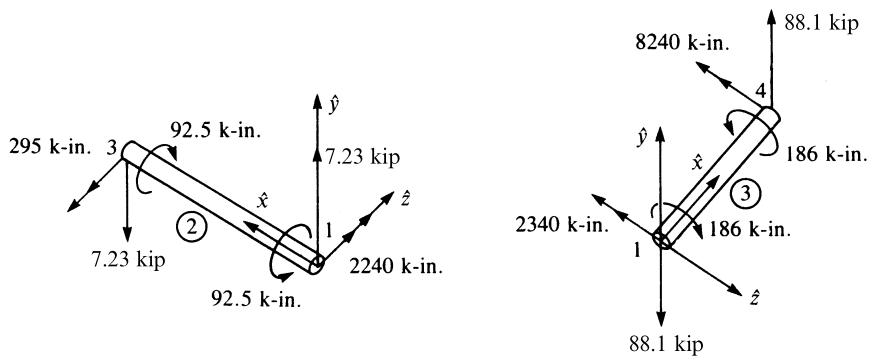$$ Free-body diagrams for all elements are shown in Figure 5–19. Each element is in equilibrium. For each element, the x^ axis is shown directed from the first node to the 

text_image

y x 186 k-in. 1260 k-in. 7.23 kip 1 2340 k-in. 1080 k-in. 19.2 kip 88.1 kip 2150 k-in. 100 kip 1960 k-in.

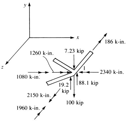
Figure 5–20 Free-body diagram of node 1 of Figure 5–18 second node, the $\hat { y }$ axis coincides with the global y axis, and the z^ axis is perpendicular to the ${ \hat { x } } { - } { \hat { y } }$ plane with its direction given by the right-hand rule. To verify equilibrium of node 1, we draw a free-body diagram of the node showing all forces and moments transferred from node 1 of each element, as in Figure 5–20. In Figure 5–20, the local forces and moments from each element have been transformed to global components, and any applied nodal forces have been included. To perform this transformation, recall that, in general, $\underline { { \hat { f } } } = \underline { { T } } \underline { { f } }$ , and therefore $\underline { { f } } =$ $\underline { { T } } ^ { T } \hat { f }$ because $\underline { T } ^ { T } = \underline { T } ^ { - 1 }$ . Since we are transforming forces at node 1 of each element, only the upper $3 \times 3$ part of Eq. (5.4.18) for $\underline { { T } } _ { G }$ need be applied. Therefore, by premultiplying the local element forces and moments at node 1 by the transpose of the transformation matrix for each element, we obtain the global nodal forces and moments as follows: # Element 1 $$ \left\{ \begin{array}{l} f _ {1 y} \\ m _ {1 x} \\ m _ {1 z} \end{array} \right\} = \left[ \begin{array}{c c c} 1 & 0 & 0 \\ 0 & - 0. 8 9 4 & - 0. 4 4 7 \\ 0 & 0. 4 4 7 & - 0. 8 9 4 \end{array} \right] \left\{ \begin{array}{l} - 1 9. 2 \\ - 1 6 7 \\ - 2 4 8 0 \end{array} \right\} $$ Simplifying, we obtain the global-coordinate force and moments as $$ f _ {1 y} = - 1 9. 2 \mathrm{kip} \quad m _ {1 x} = 1 2 6 0 \mathrm{k} \text {-in.} \quad m _ {1 z} = 2 1 5 0 \mathrm{k} \text {-in.} \tag {5.4.37} $$ where $f _ { 1 y } = \hat { f } _ { 1 \atop 1 }$ y because $y = \hat { y }$ # Element 2 $$ \left\{ \begin{array}{l} f _ {1 y} \\ m _ {1 x} \\ m _ {1 z} \end{array} \right\} = \left[ \begin{array}{c c c} 1 & 0 & 0 \\ 0 & - 0. 8 9 4 & 0. 4 4 7 \\ 0 & - 0. 4 4 7 & - 0. 8 9 4 \end{array} \right] \left\{ \begin{array}{l} 7. 2 3 \\ - 9 2. 5 \\ 2 2 4 0 \end{array} \right\} $$ Simplifying, we obtain the global-coordinate force and moments as $$ f _ {1 y} = 7. 2 3 \mathrm{kip} \quad m _ {1 x} = 1 0 8 0 \mathrm{k} \text {-in.} \quad m _ {1 z} = - 1 9 6 0 \mathrm{k} \text {-in.} \tag {5.4.38} $$ Element 3 $$ \left\{ \begin{array}{l} f _ {1 y} \\ m _ {1 x} \\ m _ {1 z} \end{array} \right\} = \left[ \begin{array}{c c c} 1 & 0 & 0 \\ 0 & 0 & 1 \\ 0 & - 1 & 0 \end{array} \right] \left\{ \begin{array}{c} - 8 8. 1 \\ 1 8 6 \\ - 2 3 4 0 \end{array} \right\} $$ Simplifying, we obtain the global-coordinate force and moments as $$ f _ {1 y} = - 8 8. 1 \mathrm{kip} \quad m _ {1 x} = - 2 3 4 0 \mathrm{k} \text {-in.} \quad m _ {1 z} = - 1 8 6 \mathrm{k} \text {-in.} \tag {5.4.39} $$ Then forces and moments from each element that are equal in magnitude but opposite in sign will be applied to node 1. Hence, the free-body diagram of node 1 is shown in Figure 5–20. Force and moment equilibrium are verified as follows: $$ \sum F _ {1 y} = - 1 0 0 - 7. 2 3 + 1 9. 2 + 8 8. 1 = 0. 0 7 \text { kip } \quad \text {(close to zero)} $$ $$ \sum M _ {1 x} = - 1 2 6 0 - 1 0 8 0 + 2 3 4 0 = 0. 0 \mathrm{k} \text {-in}. $$ $$ \sum M _ {1 z} = - 2 1 5 0 + 1 9 6 0 + 1 8 6 = - 4. 0 0 \mathrm{k} \text {-in}. \quad \text {(close to zero)} $$ Thus, we have verified the solution to be correct within the accuracy associated with a longhand solution. 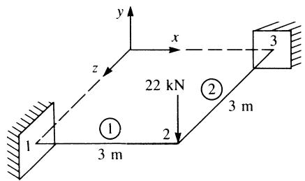# Example 5.6 Analyze the grid shown in Figure 5–21. The grid consists of two elements, is fixed at nodes 1 and 3, and is subjected to a downward vertical load of 22 kN. The globalcoordinate axes and element lengths are shown in the figure. Let $E = 2 1 0 \mathrm { \ G P a } , G =$ 84 GPa, $I = 1 6 . 6 \times 1 0 ^ { - 5 } \mathrm { m } ^ { 4 }$ , and $J = 4 . 6 \times 1 0 ^ { - 5 } ~ \mathrm { m } ^ { 4 }$ . As in Example 5.5, we use the boundary conditions and express only the part of the stiffness matrix associated with the degrees of freedom at node 2. The boundary conditions at nodes 1 and 3 are $$ d _ {1 y} = \phi_ {1 x} = \phi_ {1 z} = 0 \quad d _ {3 y} = \phi_ {3 x} = \phi_ {3 z} = 0 \tag {5.4.40} $$ 

text_image

y x z 22 kN ② 3 1 ① 2 3 m 3 m

Figure 5–21 Grid example