Similarly, from Figure 7–17, we can show that $$ [ k ^ {(2)} ] = [ k ^ {(4)} ] = \frac {E}{4 . 1 6} \left[ \begin{array}{c c c c c c} 2 & & 3 & & 5 \\ 4 & & 1 & & 5 \\ 1. 5 & - 1. 0 & - 0. 1 & 0. 2 & - 1. 4 & 0. 8 \\ & 3. 0 & - 0. 2 & - 2. 6 & 1. 2 & - 0. 4 \\ & & 1. 5 & 1. 0 & - 1. 4 & - 0. 8 \\ & & & 3. 0 & - 1. 2 & - 0. 4 \\ & & & & 2. 8 & 0. 0 \\ \text {Symmetry} & & & & & 0. 8 \end{array} \right] \tag {7.5.11} $$ where the numbers above the columns in Eqs. (7.5.10) and (7.5.11) indicate the orders of the degrees of freedom associated with each stiffness matrix. Here the quantity in the denominator of Eq. (6.4.3), $4 A ( 1 + \nu ) ( 1 - 2 \nu )$ , is equal to 4.16 in Eqs. (7.5.10) and (7.5.11) because $A = 2 \mathrm { i n } ^ { 2 }$ and n is taken to be 0.3. Also, the thickness t of the element has been taken as 1 in. Now we can superimpose the stiffness terms as indicated by Eq. (7.5.9) to obtain the general expression for a four-CST element. The resulting assembled total stiffness matrix before static condensation is applied is given by $$ [ k ] = \frac {E}{4 . 1 6} \left[ \begin{array}{c c c c c c c c c c} 3. 0 & 2. 0 & 0. 1 & 0. 2 & 0. 0 & 0. 0 & - 0. 1 & - 0. 2 & - 3. 0 & - 2. 0 \\ & 6. 0 & - 0. 2 & 2. 6 & 0. 0 & 0. 0 & 0. 2 & - 2. 6 & - 2. 0 & - 6. 0 \\ & & 3. 0 & - 2. 0 & - 0. 1 & 0. 2 & 0. 0 & 0. 0 & - 3. 0 & 2. 0 \\ & & & 6. 0 & - 0. 2 & - 2. 6 & 0. 0 & 0. 0 & 2. 0 & - 6. 0 \\ & & & & 3. 0 & 2. 0 & 0. 1 & 0. 2 & - 3. 0 & - 2. 0 \\ & & & & & 6. 0 & - 0. 2 & 2. 6 & - 2. 0 & - 6. 0 \\ & & & & & & 3. 0 & - 2. 0 & - 3. 0 & 2. 0 \\ & & & & & & & 6. 0 & 2. 0 & - 6. 0 \\ & & & & & & & & 1 2. 0 & 0. 0 \\ \text {Symmetry} & & & & & & & & & 2 4. 0 \end{array} \right] \tag {7.5.12} $$ After we partition Eq. (7.5.12) and use Eq. (7.5.6), the condensed stiffness matrix is given by $$ \left[ k _ {c} \right] = \frac {E}{4 . 1 6} \left[ \begin{array}{c c c c c c c c} u _ {1} & v _ {1} & u _ {2} & v _ {2} & u _ {3} & v _ {3} & u _ {4} & v _ {4} \\ 2. 0 8 & 1. 0 0 & - 0. 4 8 & 0. 2 0 & - 0. 9 2 & - 1. 0 0 & - 0. 6 8 & - 0. 2 0 \\ & 4. 1 7 & - 0. 2 0 & 1. 4 3 & - 1. 0 0 & - 1. 8 3 & 0. 2 0 & - 3. 7 7 \\ & & 2. 0 8 & - 1. 0 0 & - 0. 6 8 & 0. 2 0 & - 0. 9 2 & 1. 0 0 \\ & & & 4. 1 7 & - 0. 2 0 & - 3. 7 7 & 1. 0 0 & - 1. 8 3 \\ & & & & 2. 0 8 & 1. 0 0 & - 0. 4 8 & 0. 2 0 \\ & & & & & 4. 1 7 & - 0. 2 0 & 1. 4 3 \\ & & & & & & 2. 0 8 & - 1. 0 0 \\ \text {Symmetry} & & & & & & & 4. 1 7 \end{array} \right] \tag {7.5.13} $$ # 7.6 Flowchart for the Solution of Plane Stress=Strain Problems In Figure 7–18, we present a flowchart of a typical finite element process used for the analysis of plane stress and plane strain problems on the basis of the theory presented in Chapter 6. # 7.7 Computer Program Assisted Step-by-Step Solution, Other Models and Results for Plane Stress=Strain Problems In this section, we present a computer-assisted step-by-step solution of a plane stress problem, along with results of some plane stress/strain problems solved using a computer program [12]. These results illustrate the various kinds of difficult problems that can be solved using a general-purpose computer program. 

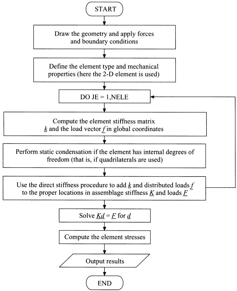
flowchart

```mermaid graph TD A["START"] --> B["Draw the geometry and apply forces and boundary conditions"] B --> C["Define the element type and mechanical properties (here the 2-D element is used)"] C --> D["DO JE = 1,NELE"] D --> E["Compute the element stiffness matrix k and the load vector f in global coordinates"] E --> F["Perform static condensation if the element has internal degrees of freedom (that is, if quadrilaterals are used)"] F --> G["Use the direct stiffness procedure to add k and distributed loads f to the proper locations in assemblage stiffness K and loads F"] G --> H["Solve Kd = F for d"] H --> I["Compute the element stresses"] I --> J["Output results"] J --> K["END"] ```

Figure 7–18 Flowchart of plane stress=strain finite element process The computer-assisted step-by-step problem is the bicycle wrench shown in Figure 7–19(a). The following steps have been used to solve for the stresses in the wrench. 1. The first step is to draw the outline of the wrench using a standard drawing program as shown in Figure 7–19(a). The exact dimensions of the wrench are obtained from Figure P7–35, where the overall depth of the wrench is 2.0 cm, the length is 14 cm, and the sides of the hexagons are 9 mm long for the middle one and 7 mm long for the side ones. The radius of the enclosed ends is 1.50 cm. 2. The second step is to use a two-dimensional mesh generator to create the model mesh as shown in Figure 7–19(b). 3. The third step is to apply the boundary conditions to the proper nodes using the proper boundary condition command. This is shown in Figure 7–19(c) as indicated by the small @ signs at the nodes on the inside of the left hexagonal shaped hole. The @ sign indicates complete fixity for a node. This means these nodes are constrained from translating in the y and z directions in the plane of the wrench. 4. The fourth step requires us to select the surface where the distributed loading is to be applied and then the magnitude of the surface traction. This is the upper surface between the middle and right hexagonal holes where the surface traction of 100 N/cm2 is applied as shown in Figure 7–19(d). In the computer program this surface changes to the color red as selected by the user (Figure 7–19(c)). 5. In step five we choose the material properties. Here ASTM A-514 steel has been selected, as this is quenched and tempered steel with high yield strength and will allow for the thickness to be minimized. 6. In step six we select the element type for the kind of analysis to be performed. Here we select the plane stress element, as this is a good approximation to the kind of behavior that is produced in a plane stress analysis. For the plane stress element a thickness is required. An initial guess of one cm is made. This thickness appears to be compatible with the other dimensions of the wrench. 7. The seventh step is an optional check of the model. If you choose to perform this step you will see the boundary conditions now appear as triangles at the left nodes corresponding to the @ signs for full fixity and the surface traction arrows, indicating the location and direction of the surface traction shown also in Figure 7–19(d). 8. In step eight we perform the stress analysis of the model. 9. In step nine we select the results, such as the displacement plot, the principal stress plot, and the von Mises stress plot. The von Mises stress plot is used to determine the failure of the wrench based on the maximum distortion energy theory as described in Section 6.5. The von Mises stress plot is shown in Figure 7–19(e). 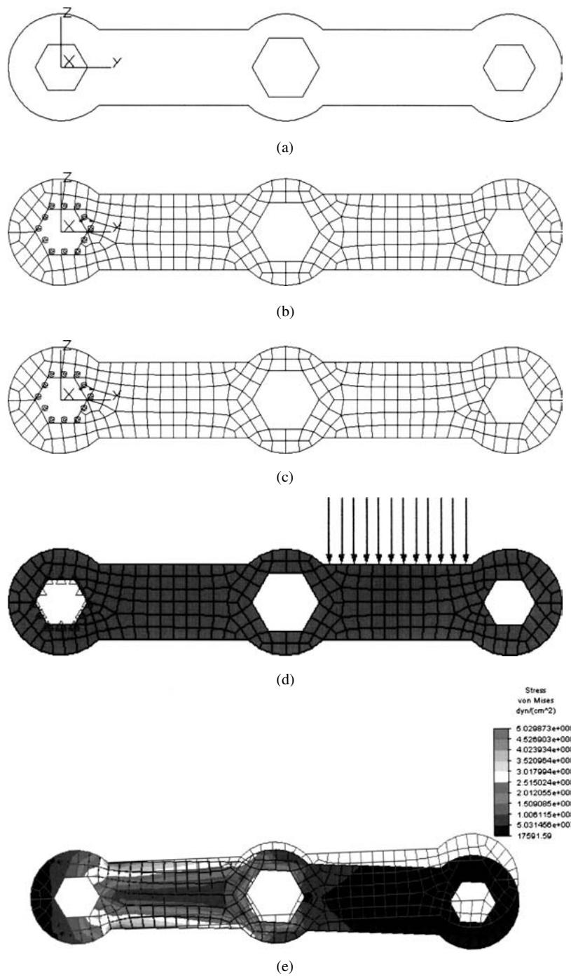The maximum von Mises stress indicated in Figure 7–19(e) is 502 MPa, and the yield  Figure 7–19 Bicycle wrench (a) Outline drawing of wrench, (b) meshed model of wrench, (c) boundary conditions and selecting surface where surface traction will be applied, (d) checked model showing the boundary conditions and surface traction, and (e) von Mises stress plot (compliments of Angela Moe) 

text_image

1000 lb 1000 lb 1000 lb (a)


heatmap

| Load Case | Maximum Value | Stress Value | |-----------|---------------|--------------| | 1 of 1 | 12050.9 | 12050.93 | | 1 of 1 | -147793e-011 | -147793e-011 |

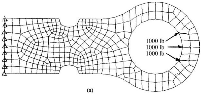
Figure 7–20 (a) Connecting rod subjected to tensile loading and (b) resulting principal stress throughout the rod strength of the ASTM A-514 steel is 690 MPa. Therefore, the wrench is safe from yielding. Additional trials can be made if the factor of safety is satisfied and if the maximum deflection appears to be satisfactory. Figure 7–20(a) shows a finite element model of a steel connecting rod that is fixed on its left edge and loading around the right inner edge of the hole with a total force of 3000 lb. For more details, including the geometry of this rod, see Figure P7–11 at the end of this chapter. Figure 7–20(b) shows the resulting maximum 

text_image

Load Case: 1 of 1 Maximum Value: 1.78441e+038 N/(m^2) Minimum Value: 282983 N/(m^2)

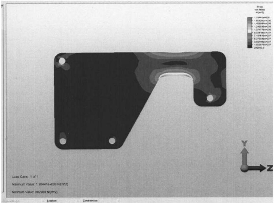
Figure 7–21 von Mises stress plot of overload protection device principal stress plot. The largest principal stress of 12051 psi occurs at the top and bottom inside edge of the hole. Figure 7–21 shows a finite element model along with the von Mises stress plot of an overload protection device (see Problem 7–30 for details of this problem). The upper member of the device was modeled. Node S at the shear pin location was constrained from vertical motion and a node at the roller E was constrained in the horizontal direction. An equilibrium load was applied at B along line BD. The magnitude of this load was calculated as one that just makes the shear stress reach 40 MPa in the pin at S. The largest von Mises stress of 178 MPa occurs at the inner edge of the cutout section. 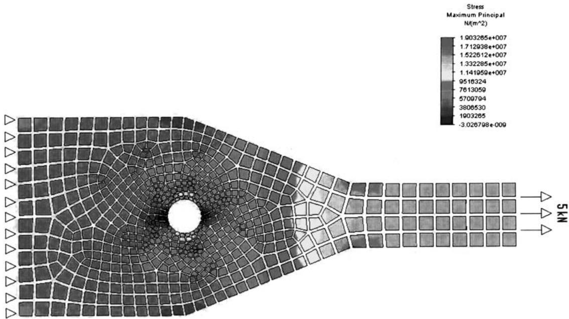Figure 7–22 shows the shrink plot of a finite element analysis of a tapered plate with a hole in it, subjected to tensile loading along the right edge. The left edge was fixed. For details of this problem see Problem 7–23. The shrink plot separates the elements for a clear look at the model. The largest principal stress of 19.0 e6 Pa (19.0 MPa) occurs at the edge of the hole, whereas the second largest principal stress of 17.95 e6 Pa (17.95 MPa) occurs at the elbow between the smallest cross section and where the taper begins. 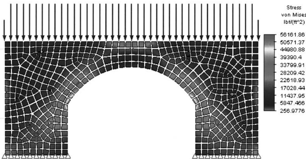Figure 7–23 shows the shrink fit plot of the maximum principal stresses in an overpass subjected to vertical loading on the top edge. The largest principal stress of 56162 lb/ft2 (390 psi) occurs at the top inside edge. For more details of this problem see Problem 7.20. 

heatmap

| Stress (m²) | Value | | ------------------ | ------------------ | | 1.903285e+007 | 1.903285e+007 | | 1.712938e+007 | 1.712938e+007 | | 1.522612e+007 | 1.522612e+007 | | 1.332285e+007 | 1.332285e+007 | | 1.141959e+007 | 1.141959e+007 | | 9516324 | 9516324 | | 7613059 | 7613059 | | 5709794 | 5709794 | | 3806530 | 3806530 | | 1903265 | 1903265 | | -3.026798e-009 | -3.026798e-009 |

Figure 7–22 Shrink fit plot of principal stresses in a tapered plate with hole Finally, Figure 7–24(a) shows a finite element discretized model of a steel spur gear for stress analysis. The auto meshing feature resulted in very small elements at the base of the tooth. The applied load of 164.8 lb and the fixed nodes around the inner hole of the gear are shown. Figure 7–24(b) shows an enlarged von Mises stress 

heatmap

| Stress von Mises Ibt/(ft^2) | | --------------------------- | | 56161.86 | | 50571.37 | | 44980.88 | | 39390.4 | | 33799.91 | | 28209.42 | | 22618.93 | | 17028.44 | | 11437.95 | | 5847.466 | | 256.9776 |

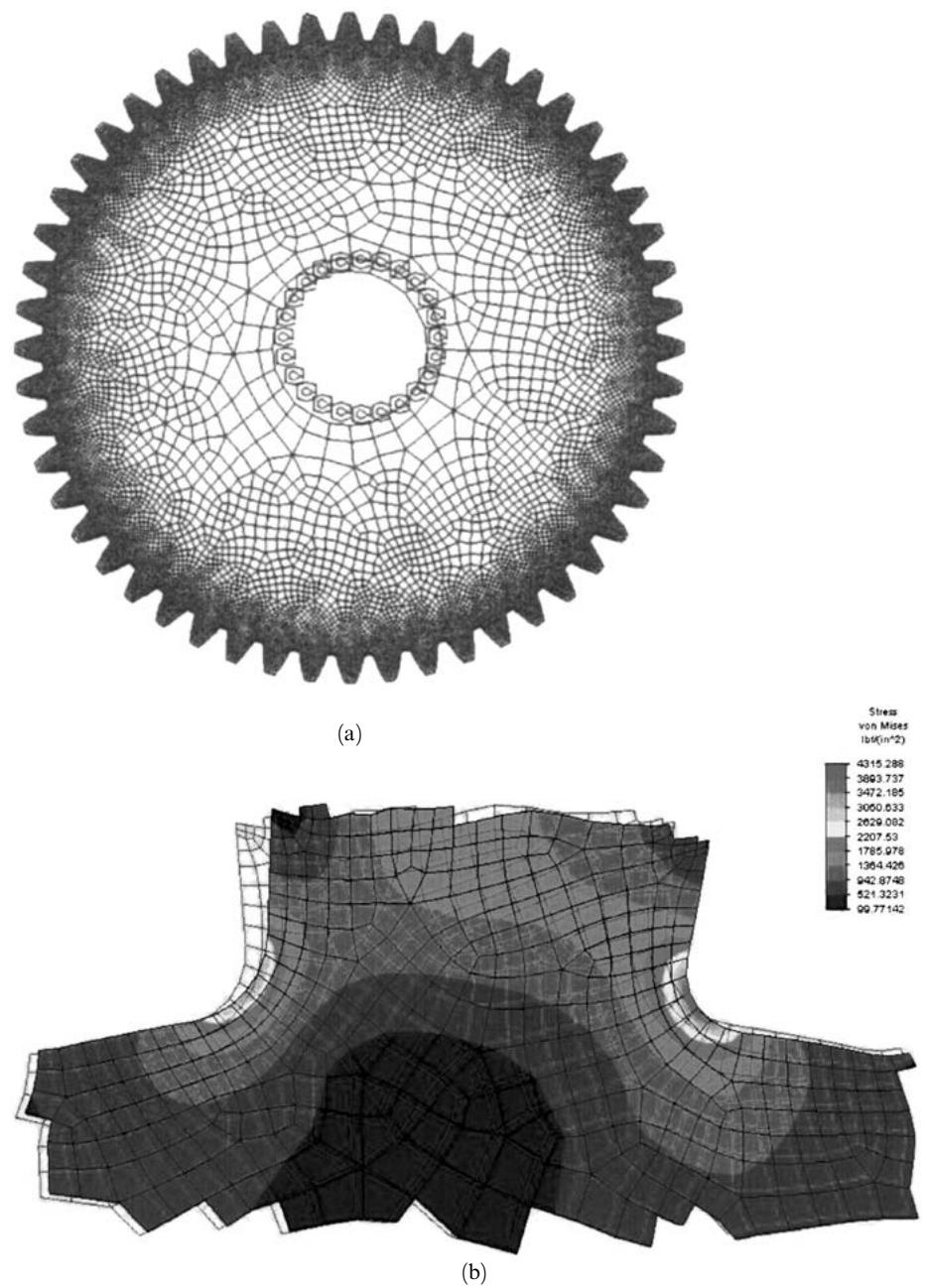
Figure 7–23 Shrink fit plot of principal stresses in overpass (Compliments of David Walgrave)  Figure 7–24 (a) Finite element model of a spur gear and (b) von Mises stress plot (Compliments of Bruce Figi) plot near the root of the tooth with the applied load acting on it. Notice that the largest stress of 4315 psi occurs at the left root of the tooth. The gear model has 27761 plane stress elements. # References [1] Desai, C. S., and Abel, J. F., Introduction to the Finite Element Method, Van Nostrand Reinhold, New York, 1972. [2] Timoshenko, S., and Goodier, J., Theory of Elasticity, 3rd ed., McGraw-Hill, New York, 1970. [3] Glockner, P. G., ‘‘Symmetry in Structural Mechanics,’’ Journal of the Structural Division, American Society of Civil Engineers, Vol. 99, No. ST1, pp. 71–89, 1973. [4] Yamada, Y., ‘‘Dynamic Analysis of Civil Engineering Structures,’’ Recent Advances in Matrix Methods of Structural Analysis and Design, R. H. Gallagher, Y. Yamada, and J. T. Oden, eds., University of Alabama Press, Tuscaloosa, AL, pp. 487–512, 1970. [5] Koswara, H., A Finite Element Analysis of Underground Shelter Subjected to Ground Shock Load, M. S. Thesis, Rose-Hulman Institute of Technology, Terre Haute, IN, 1983. [6] Dunlop, P., Duncan, J. M., and Seed, H. B., ‘‘Finite Element Analyses of Slopes in Soil,’’ Journal of the Soil Mechanics and Foundations Division, Proceedings of the American Society of Civil Engineers, Vol. 96, No. SM2, March 1970. [7] Cook, R. D., Malkus, D. S., Plesha, M. E., and Witt, R. J., Concepts and Applications of Finite Element Analysis, 4th ed., Wiley, New York, 2002. [8] Taylor, R. L., Beresford, P. J., and Wilson, E. L., ‘‘A Nonconforming Element for Stress Analysis,’’ International Journal for Numerical Methods in Engineering, Vol. 10, No. 6, pp. 1211–1219, 1976. [9] Melosh, R. J., ‘‘Basis for Derivation of Matrices for the Direct Stiffness Method,’’ Journal of the American Institute of Aeronautics and Astronautics, Vol. 1, No. 7, pp. 1631–1637. July 1963. [10] Fraeijes de Veubeke, B., ‘‘Upper and Lower Bounds in Matrix Structural Analysis,’’ Matrix Methods of Structural Analysis, AGARDograph 72, B. Fraeijes de Veubeke, ed., Macmillan, New York, 1964. [11] Dunder, V., and Ridlon, S., ‘‘Practical Applications of Finite Element Method,’’ Journal of the Structural Division, American Society of Civil Engineers, No. ST1, pp. 9–21, 1978. [12] Linear Stress and Dynamics Reference Division, Docutech On-line Documentation, Algor, Inc., Pittsburgh, PA 15238. [13] Bettess, P., ‘‘More on Infinite Elements,’’ International Journal for Numerical Methods in Engineering, Vol. 15, pp. 1613–1626, 1980. [14] Gere, J. M., Mechanics of Materials, 5th ed., Brooks/Cole Publishers, Pacific Grove, CA, 2001. [15] Superdraw Reference Division, Docutech On-line Documentation, Algor, Inc., Pittsburgh, PA 15238. [16] Cook, R. D., and Young, W. C., Advanced Mechanics of Materials, Macmillan, New York, 1985. [17] Cook, R. D., Finite Element Modeling for Stress Analysis, Wiley, New York, 1995. [18] Kurowski, P., ‘‘Easily Made Errors Mar FEA Results,’’ Machine Design, Sept. 13, 2001. [19] Huebner, K. H., Dewirst, D. L., Smith, D. E., and Byrom, T. G., The Finite Element Method for Engineers, Wiley, New York, 2001. [20] Demkowicz, L., Devloo, P., and Oden, J. T., ‘‘On an h-Type Mesh-Refinement Strategy Based on Minimization of Interpolation Errors,’’ Comput. Methods Appl. Mech. Eng., Vol. 53, 1985, pp. 67–89. [21] Lo¨hner, R., Morgan, K., and Zienkiewicz, O. C., ‘‘An Adaptive Finite Element Procedure for Compressible High Speed Flows,’’ Comput. Methods Appl. Mech. Eng., Vol. 51, 1985, pp. 441–465. [22] Lo¨hner, R., ‘‘An Adaptive Finite Element Scheme for Transient Problems in CFD,’’ Comput. Methods Appl. Mech. End., Vol. 61, 1987, pp. 323–338. [23] Ramakrishnan, R., Bey, K. S., and Thornton, E. A., ‘‘Adaptive Quadrilateral and Triangular Finite Element Scheme for Compressible Flows,’’ AIAA J., Vol. 28, No. 1, 1990, pp. 51–59. [24] Peano, A. G., ‘‘Hierarchies of Conforming Finite Elements for Plane Elasticity and Plate Bending,’’ Comput. Match. Appl., Vol. 2, 1976, pp. 211–224. [25] Szabo´, B. A., ‘‘Some Recent Developments in Finite Element Analysis,’’ Comput. Match. Appl., Vol. 5, 1979, pp. 99–115. [26] Peano, A. G., Pasini, A., Riccioni., R. and Sardella, L., ‘‘Adaptive Approximation in Finite Element Structural Analysis,’’ Comput. Struct., Vol. 10, 1979, pp. 332–342. [27] Zienkiewicz, O. C., Gago, J. P. de S. R., and Kelly, D. W., ‘‘The Hierarchical Concept in Finite Element Analysis,’’ Comput. Struct., Vol. 16, No. 1–4, 1983, pp. 53–65. [28] Szabo´ , B. A., ‘‘Mesh Design for the p-Version of the Finite Element Method,’’ Comput. Methods Appl. Mech. Eng., Vol. 55, 1986, pp. 181–197. [29] Toogood, Roger, Pro/MECHANICA, Structural Tutorial, SDC Publications, 2001. 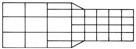# d Problems 7.1 For the finite element mesh shown in Figure P7–1, comment on the goodness of the mesh. Indicate the mistakes in the model. Explain and show how to correct them. 

natural_image

Pure geometric grid pattern with no text, numbers, or symbols

Figure P7–1 

text_image

C A D B

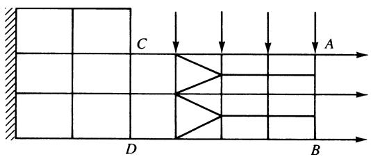
Figure P7–2 7.2 Comment on the mesh sizing in Figure P7–2. Is it reasonable? If not, explain why not. 7.3 What happens if the material property n ¼ 0:5 in the plane strain case? Is this possible? Explain. 7.4 Under what conditions is the structure in Figure P7–4 a plane strain problem? Under what conditions is the structure a plane stress problem?