text_image

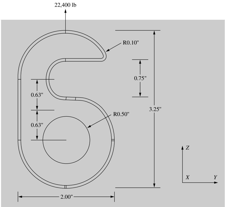
22,400 lb R0.10" 0.75" 0.63" 0.63" R0.50" 3.25" 2.00" Z X Y

Figure P7–28 

text_image

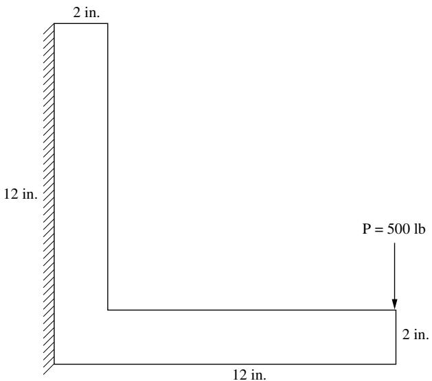
2 in. 12 in. 12 in. P = 500 lb 2 in.

Figure P7–29 

text_image

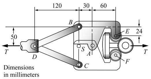
120 30 60 50 T D B E 24 S A C F T Dimensions in millimeters


text_image

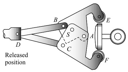
Released position

Figure P7–30 Overload protection device 

text_image

24 4 5 12.5 7000 lb 4 5 24 Dimensions in inches

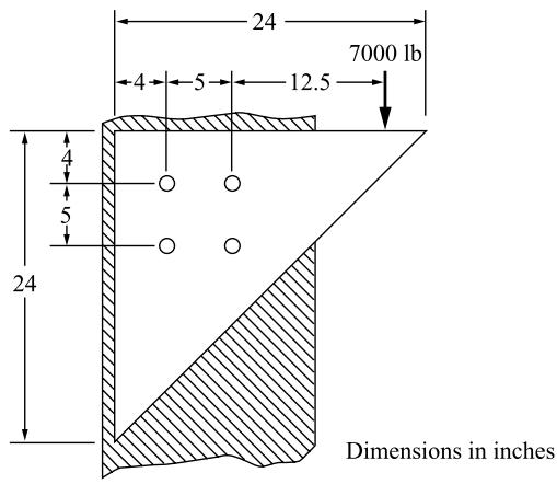
Figure P7–31 Steel triangular plate connection 

text_image

1000 lb 5 3.5 2.5 A B 1.5 C 1.0 0.5r 8 Dimensions in inches

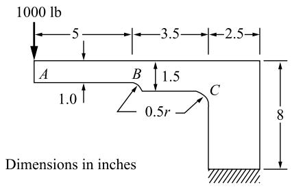
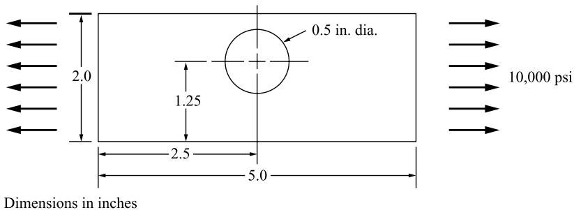
Figure P7-32 Machine part  7.33 A plate with a hole off-centered is shown in Figure P7–33. Determine how close to the top edge the hole can be placed before yielding of the A36 steel occurs (based on the maximum distortion energy theory). The applied tensile stress is 10,000 psi, and the plate thickness is $\frac{1}{4}$ in. Now if the plate is made of 6061-T6 aluminum alloy with a yield strength of 37 ksi, does this change your answer? If the plate thickness is changed to $\frac{1}{2}$ in., how does this change the results? Use same total load as when the plate is $\frac{1}{4}$ in. thick. 

text_image

2.0 1.25 0.5 in. dia. 2.5 5.0 10,000 psi Dimensions in inches

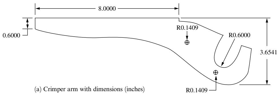
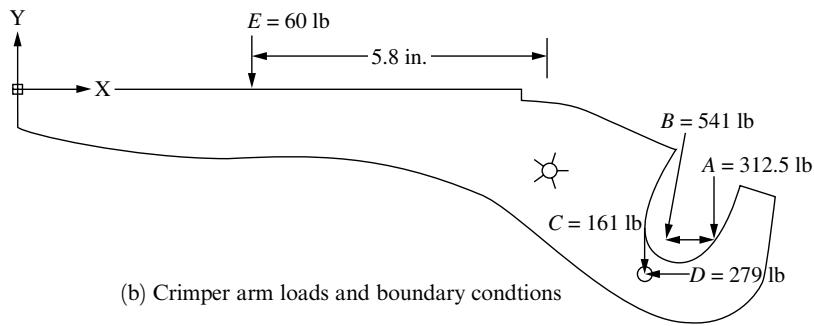
Figure P7–33 Plate with off-centered hole  7.34 One arm of a crimper tool shown in Figure P7–34 is to be designed of 1080 as-rolled steel. The loads and boundary conditions are shown in the figure. Select a thickness for the arm based on the material not yielding with a factor of safety of 1.5. Recommend any other changes in the design. (Scale any other dimensions that you need.) 

text_image

(a) Crimper arm with dimensions (inches)


text_image

Y E = 60 lb 5.8 in. X B = 541 lb A = 312.5 lb C = 161 lb D = 279 lb (b) Crimper arm loads and boundary conditions

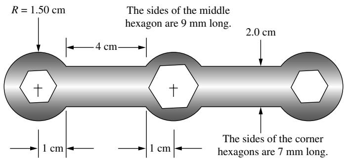
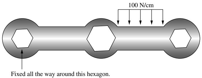
Figure P7–34 Crimper arm  7.35 Design the bicycle wrench with the approximate dimensions shown in Figure P7–35. If you need to change dimensions explain why. The wrench should be made of steel or aluminum alloy. Determine the thickness needed based on the maximum distortion energy theory. Plot the deformed shape of the wrench and the principal stress and von Mises stress. The boundary conditions are shown in the figure, and the loading is shown as a distributed load acting over the right part of the wrench. Use a factor of safety of 1.5 against yielding. 

text_image

R = 1.50 cm 4 cm The sides of the middle hexagon are 9 mm long. 2.0 cm 1 cm 1 cm The sides of the corner hexagons are 7 mm long.


text_image

100 N/cm Fixed all the way around this hexagon.

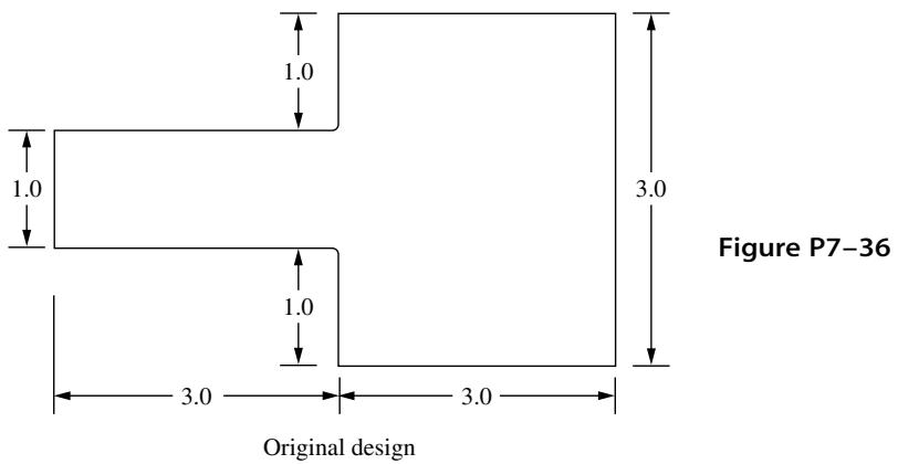
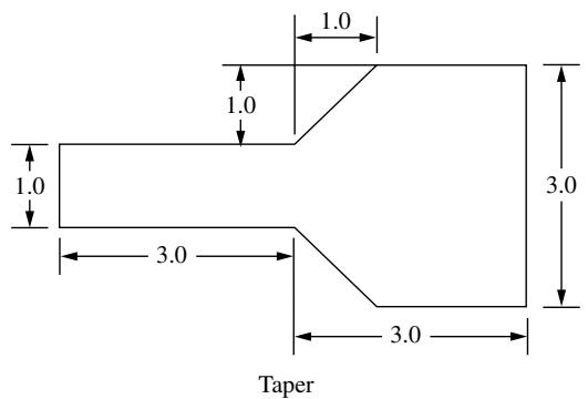
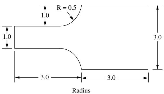
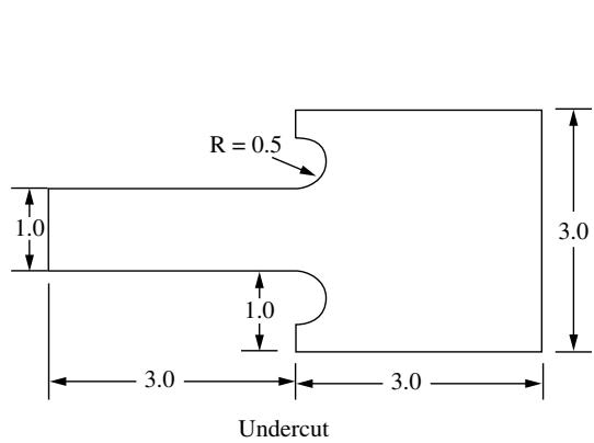
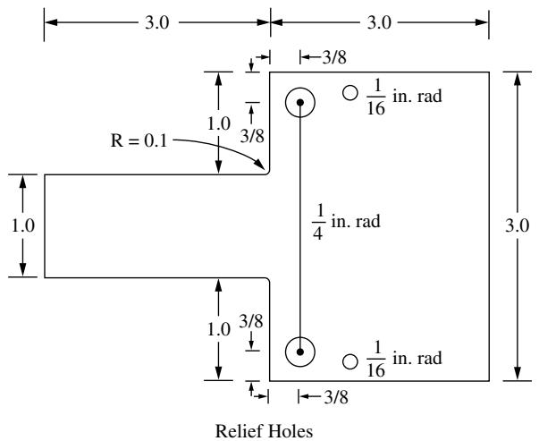
Figure P7–35 Bicycle wrench  7.36 For the various parts shown in Figure P7–36 determine the best one to relieve stress. Make the original part have a small radius of 0.1 in. at the inside re-entrant corners. Place a uniform pressure load of 1000 psi on the right end of each part and fix the left end. All units shown are taken in inches. Let the material be A 36 steel. 

text_image

1.0 1.0 3.0 1.0 3.0 3.0 Figure P7-36 Original design


text_image

1.0 1.0 1.0 3.0 3.0 3.0 Taper


text_image

R = 0.5 1.0 1.0 3.0 3.0 3.0 Radius


text_image

R = 0.5 1.0 1.0 3.0 3.0 3.0 Undercut


text_image

3.0 3.0 3/8 R = 0.1 1.0 3/8 1/4 in. rad 1/16 in. rad 3.0 1.0 3/8 1.0 3/8 3/8 Relief Holes

Figure P7–36 ðContinuedÞ # Development of the Linear-Strain Triangle Equations # Introduction In this chapter, we consider the development of the stiffness matrix and equations for a higher-order triangular element, called the linear-strain triangle (LST). This element is available in many commercial computer programs and has some advantages over the constant-strain triangle described in Chapter 6. The LST element has six nodes and twelve unknown displacement degrees of freedom. The displacement functions for the element are quadratic instead of linear (as in the CST). The procedures for development of the equations for the LST element follow the same steps as those used in Chapter 6 for the CST element. However, the number of equations now becomes twelve instead of six, making a longhand solution extremely cumbersome. Hence, we will use a computer to perform many of the mathematical operations. After deriving the element equations, we will compare results from problems solved using the LST element with those solved using the CST element. The introduction of the higher-order LST element will illustrate the possible advantages of higherorder elements and should enhance your general understanding of the concepts involved with finite element procedures. # 8.1 Derivation of the Linear-Strain Triangular Element Stiffness Matrix and Equations We will now derive the LST stiffness matrix and element equations. The steps used here are identical to those used for the CST element, and much of the notation is the same. 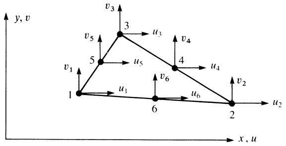# Step 1 Select Element Type Consider the triangular element shown in Figure 8–1 with the usual end nodes and three additional nodes conveniently located at the midpoints of the sides. Thus, a computer program can automatically compute the midpoint coordinates once the coordinates of the corner nodes are given as input. 

text_image

y, v v3 v5 3 u3 v4 v1 5 u5 4 u4 v6 v2 1 u1 u6 6 2 u2 x, u

Figure 8–1 Basic six-node triangular element showing degrees of freedom The unknown nodal displacements are now given by $$ \{d \} = \left\{ \begin{array}{l} \underline {{d}} _ {1} \\ \underline {{d}} _ {2} \\ \underline {{d}} _ {3} \\ \underline {{d}} _ {4} \\ \underline {{d}} _ {5} \\ \underline {{d}} _ {6} \end{array} \right\} = \left\{ \begin{array}{l} u _ {1} \\ v _ {1} \\ u _ {2} \\ v _ {2} \\ u _ {3} \\ v _ {3} \\ u _ {4} \\ v _ {4} \\ u _ {5} \\ v _ {5} \\ u _ {6} \\ v _ {6} \end{array} \right\} \tag {8.1.1} $$ # Step 2 Select a Displacement Function We now select a quadratic displacement function in each element as $$ u (x, y) = a _ {1} + a _ {2} x + a _ {3} y + a _ {4} x ^ {2} + a _ {5} x y + a _ {6} y ^ {2} \tag {8.1.2} $$ $$ v (x, y) = a _ {7} + a _ {8} x + a _ {9} y + a _ {1 0} x ^ {2} + a _ {1 1} x y + a _ {1 2} y ^ {2} $$ Again, the number of coefficients $a _ { i } ( 1 2 )$ equals the total number of degrees of freedom for the element. The displacement compatibility among adjoining elements is satisfied because three nodes are located along each side and a parabola is defined by three points on its path. Since adjacent elements are connected at common nodes, their displacement compatibility across the boundaries will be maintained. In general, when considering triangular elements, we can use a complete polynomial in Cartesian coordinates to describe the displacement field within an element.

Terms in Pascal Triangle	Polynomial Degree	Number of Terms	Triangle
1	0 (constant)	1
x y	1 (linear)	3	CST (Chap. 6)
$x^{2}$ $xy$ $y^{2}$	2 (quadratic)	6
$x^{3}$ $x^{2}y$ $xy^{2}$ $y^{3}$	3 (cubic)	10

Figure 8–2 Relation between type of plane triangular element and polynomial coefficients based on a Pascal triangle Using internal nodes as necessary for the higher-order cubic and quartic elements, we use all terms of a truncated Pascal triangle in the displacement field or, equivalently, the shape functions, as shown by Figure 8–2; that is, a complete linear function is used for the CST element considered previously in Chapter 6. The complete quadratic function is used for the LST of this chapter. The complete cubic function is used for the quadratic-strain triangle (QST), with an internal node necessary as the tenth node. The general displacement functions, Eqs. (8.1.2), expressed in matrix form are now $$ \{\psi \} = \left\{ \begin{array}{l} u \\ v \end{array} \right\} = \left[ \begin{array}{c c c c c c c c c c c c} 1 & x & y & x ^ {2} & x y & y ^ {2} & 0 & 0 & 0 & 0 & 0 & 0 \\ 0 & 0 & 0 & 0 & 0 & 0 & 1 & x & y & x ^ {2} & x y & y ^ {2} \end{array} \right] \left\{ \begin{array}{l} a _ {1} \\ a _ {2} \\ \vdots \\ a _ {1 2} \end{array} \right\} \tag {8.1.3} $$ Alternatively, we can express Eq. (8.1.3) as $$ \{\psi \} = [ M ^ {*} ] \{a \} \tag {8.1.4} $$ where $[ M ^ { * } ]$ is defined to be the first matrix on the right side of Eq. (8.1.3). The coefficients $a _ { 1 }$ through $a _ { 1 2 }$ can be obtained by substituting the coordinates into u and v as follows: $$ \left\{ \begin{array}{l} u _ {1} \\ u _ {2} \\ \vdots \\ u _ {6} \\ v _ {1} \\ \vdots \\ v _ {5} \\ v _ {6} \end{array} \right\} = \left[ \begin{array}{c c c c c c c c c c c c c} 1 & x _ {1} & y _ {1} & x _ {1} ^ {2} & x _ {1} y _ {1} & y _ {1} ^ {2} & 0 & 0 & 0 & 0 & 0 & 0 \\ 1 & x _ {2} & y _ {2} & x _ {2} ^ {2} & x _ {2} y _ {2} & y _ {2} ^ {2} & 0 & 0 & 0 & 0 & 0 & 0 \\ \vdots & \vdots & \vdots & \vdots & \vdots & \vdots & \vdots & \vdots & \vdots & \vdots & \vdots & \vdots \\ 1 & x _ {6} & y _ {6} & x _ {6} ^ {2} & x _ {6} y _ {6} & y _ {6} ^ {2} & 0 & 0 & 0 & 0 & 0 & 0 \\ 0 & 0 & 0 & 0 & 0 & 0 & 1 & x _ {1} & y _ {1} & x _ {1} ^ {2} & x _ {1} y _ {1} & y _ {1} ^ {2} \\ \vdots & \vdots & \vdots & \vdots & \vdots & \vdots & \vdots & \vdots & \vdots & \vdots & \vdots & \vdots \\ 0 & 0 & 0 & 0 & 0 & 0 & 1 & x _ {5} & y _ {5} & x _ {5} ^ {2} & x _ {5} y _ {5} & y _ {5} ^ {2} \\ 0 & 0 & 0 & 0 & 0 & 0 & 1 & x _ {6} & y _ {6} & x _ {6} ^ {2} & x _ {6} y _ {6} & y _ {6} ^ {2} \end{array} \right] \left\{ \begin{array}{l} a _ {1} \\ a _ {2} \\ \vdots \\ a _ {6} \\ a _ {7} \\ \vdots \\ a _ {1 1} \\ a _ {1 2} \end{array} \right\} \tag {8.1.5} $$ Solving for the $\boldsymbol { a } _ { i } { \widetilde { \mathbf { s } } } ,$ we have $$ \left\{ \begin{array}{c} a _ {1} \\ \vdots \\ a _ {6} \\ a _ {7} \\ \vdots \\ a _ {1 2} \end{array} \right\} = \left[ \begin{array}{c c c c c c c c c c c c c} 1 & x _ {1} & y _ {1} & x _ {1} ^ {2} & x _ {1} y _ {1} & y _ {1} ^ {2} & 0 & 0 & 0 & 0 & 0 & 0 \\ \vdots & \vdots & \vdots & \vdots & \vdots & \vdots & \vdots & \vdots & \vdots & \vdots & \vdots & \vdots \\ 1 & x _ {6} & y _ {6} & x _ {6} ^ {2} & x _ {6} y _ {6} & y _ {6} ^ {2} & 0 & 0 & 0 & 0 & 0 & 0 \\ 0 & 0 & 0 & 0 & 0 & 0 & 1 & x _ {1} & y _ {1} & x _ {1} ^ {2} & x _ {1} y _ {1} & y _ {1} ^ {2} \\ \vdots & \vdots & \vdots & \vdots & \vdots & \vdots & \vdots & \vdots & \vdots & \vdots & \vdots & \vdots \\ 0 & 0 & 0 & 0 & 0 & 0 & 1 & x _ {6} & y _ {6} & x _ {6} ^ {2} & x _ {6} y _ {6} & y _ {6} ^ {2} \end{array} \right] ^ {- 1} \left\{ \begin{array}{c} u _ {1} \\ \vdots \\ u _ {6} \\ v _ {1} \\ \vdots \\ v _ {6} \end{array} \right\} \tag {8.1.6} $$ or, alternatively, we can express Eq. (8.1.6) as $$ \{a \} = [ X ] ^ {- 1} \{d \} \tag {8.1.7} $$ where ½X is the $1 2 \times 1 2$ matrix on the right side of Eq. (8.1.6). It is best to invert the ½X matrix by using a digital computer. Then the $\vec { a _ { i } \mathrm { s , } }$ in terms of nodal displacements, are substituted into Eq. (8.1.4). Note that only the $6 \times 6$ part of ½X in Eq. (8.1.6) really must be inverted. Finally, using Eq. (8.1.7) in Eq. (8.1.4), we can obtain the general displacement expressions in terms of the shape functions and the nodal degrees of freedom as $$ \{\psi \} = [ N ] \{d \} \tag {8.1.8} $$ where $[ N ] = [ M ^ { * } ] [ X ] ^ { - 1 }$ ð8:1:9Þ # Step 3 Define the Strain=Displacement and Stress=Strain Relationships The element strains are again given by $$ \{\varepsilon \} = \left\{ \begin{array}{l} \varepsilon_ {x} \\ \varepsilon_ {y} \\ \gamma_ {x y} \end{array} \right\} = \left\{ \begin{array}{c} \frac {\partial u}{\partial x} \\ \frac {\partial v}{\partial y} \\ \frac {\partial v}{\partial x} + \frac {\partial u}{\partial y} \end{array} \right\} \tag {8.1.10} $$ or, using Eq. (8.1.3) for u and v in Eq. (8.1.10), we obtain $$ \{\varepsilon \} = \left[ \begin{array}{c c c c c c c c c c c c} 0 & 1 & 0 & 2 x & y & 0 & 0 & 0 & 0 & 0 & 0 & 0 \\ 0 & 0 & 0 & 0 & 0 & 0 & 0 & 0 & 1 & 0 & x & 2 y \\ 0 & 0 & 1 & 0 & x & 2 y & 0 & 1 & 0 & 2 x & y & 0 \end{array} \right] \left\{ \begin{array}{l} a _ {1} \\ a _ {2} \\ \vdots \\ a _ {1 2} \end{array} \right\} \tag {8.1.11} $$ We observe that $\operatorname { E q . }$ (8.1.11) yields a linear strain variation in the element. Therefore, the element is called a linear-strain triangle (LST). Rewriting Eq. (8.1.11), we have $$ \{\varepsilon \} = [ M ^ {\prime} ] \{a \} \tag {8.1.12} $$ where $[ M ^ { \prime } ]$ is the first matrix on the right side of Eq. (8.1.11). Substituting Eq. (8.1.6) for the $\boldsymbol { a } _ { i } { } ^ { \prime } \boldsymbol { \mathbf { s } }$ into Eq. (8.1.12), we have $\{ \varepsilon \}$ in terms of the nodal displacements as $$ \{\varepsilon \} = [ B ] \{d \} \tag {8.1.13} $$ where $[ B ]$ is a function of the variables x and y and the coordinates $( x _ { 1 } , y _ { 1 } )$ through $( x _ { 6 } , y _ { 6 } )$ given by $$ [ B ] = [ M ^ {\prime} ] [ X ] ^ {- 1} \tag {8.1.14} $$ where Eq. (8.1.7) has been used in expressing Eq. (8.1.14). Note that ½B is now a matrix of order $3 \times 1 2$ . The stresses are again given by $$ \left\{ \begin{array}{l} \sigma_ {x} \\ \sigma_ {y} \\ \tau_ {x y} \end{array} \right\} = [ D ] \left\{ \begin{array}{l} \varepsilon_ {x} \\ \varepsilon_ {y} \\ \gamma_ {x y} \end{array} \right\} = [ D ] [ B ] \{d \} \tag {8.1.15} $$ where ½D is given by Eq. (6.1.8) for plane stress or by Eq. (6.1.10) for plane strain. These stresses are now linear functions of x and y coordinates. # Step 4 Derive the Element Stiffness Matrix and Equations We determine the stiffness matrix in a manner similar to that used in Section 6.2 by using Eq. (6.2.50) repeated here as $$ [ k ] = \iiint_ {V} [ B ] ^ {T} [ D ] [ B ] d V \tag {8.1.16} $$ However, the ½B matrix is now a function of x and y as given by Eq. (8.1.14). Therefore, we must perform the integration in Eq. (8.1.16). Finally, the ½B matrix is of the form $$ [ B ] = \frac {1}{2 A} \left[ \begin{array}{c c c c c c c c c c c c} \beta_ {1} & 0 & \beta_ {2} & 0 & \beta_ {3} & 0 & \beta_ {4} & 0 & \beta_ {5} & 0 & \beta_ {6} & 0 \\ 0 & \gamma_ {1} & 0 & \gamma_ {2} & 0 & \gamma_ {3} & 0 & \gamma_ {4} & 0 & \gamma_ {5} & 0 & \gamma_ {6} \\ \gamma_ {1} & \beta_ {1} & \gamma_ {2} & \beta_ {2} & \gamma_ {3} & \beta_ {3} & \gamma_ {4} & \beta_ {4} & \gamma_ {5} & \beta_ {5} & \gamma_ {6} & \beta_ {6} \end{array} \right] \tag {8.1.17} $$ where the $\beta \mathrm { ^ { * } s }$ and $\gamma \mathbf { \bar { s } }$ are now functions of x and y as well as of the nodal coordinates, as is illustrated for a specific linear-strain triangle in Section 8.2 by Eq. (8.2.8). The stiffness matrix is then seen to be a 12 12 matrix on multiplying the matrices in Eq. (8.1.16). The stiffness matrix, Eq. (8.1.16), is very cumbersome to obtain in explicit form, so it will not be given here. However, if the origin of the coordinates is considered to be at the centroid of the element, the integrations become amenable [9]. Alternatively, area coordinates [3, 8, 9] can be used to obtain an explicit form of the stiffness matrix. However, even the use of area coordinates usually involves tedious calculations. Therefore, the integration is best carried out numerically. (Numerical integration is described in Section 10.4.)