Free convection, 538, 540
Fringe carpet, 369
Functional, defined, 12
# G
Galerkin’s method, 12–13, 124–127, 131, 201–203
bar element formulation, 125–127
beam element equations, 201–203
general formulation, 124–125
one-dimensional bar element equations, 124–127, 131
residual method, 124–127, 131 use of, 12–13
Gauss-Jordan method, 718–720
Gauss-Seidel iteration, 733–735
Gaussian elimination, 726–733
Gaussian quadrature, 463–466, 469–475
element stresses, evaluation of, 473–475
one-point, 463–464
sti¤ness matrix, evaluation of, 469–473
three-point, 465–466
two-point formula, 464–465
Global equations, 13–14, 34, 70, 161–163, 320–322, 601
assemblage of, 13–14
bar element, 70
beam element, 161–163
constant-strain triangular (CST) element, 320–322
fluid flow, 601
spring element, 34
Global sti¤ness matrix, 36, 78–81. See also Total sti¤ness matrix
bar element, 78–81
inverse, 80
spring assembly, 36
transverse, 80
Gradient/potential relationship, 599, 607
Grid, defined, 238
Grid equations, 214, 238–255
determination of, 238–255
introduction to, 214
open sections, 241
polar moment of inertia, 240
torsional constant, 240–241, 242
# H
h method of refinement, 355–356
Harmonic motion, simple, 649
Heat flux, 542, 546
Heat flux/temperature gradient relationship, 542, 556–557
Heat transfer, 534–593, 686–693
coe‰cients, 539–540
convection, 538–539, 540
di¤erential equations, 535–538
element conduction matrix, 542–546, 557–558
finite element formulation, 540–555, 555–564, 566–568, 569–574
flowchart for, 574
Galerkin’s method, 569–574
heat conduction, one-dimensional, 535–537
heat conduction, two-dimensional, 537–538
heat flux/temperature gradient relationship, 542, 556–557
heat-transfer coe‰cients, 539–540
introduction to, 534–535
line sources, 564–566
mass transport, 569–574
nodal temperature, 546
numerical time integration, 687–683
one-dimensional, 540–555, 569
point sources, 564–566
program, examples of, 574–576
temperature function, 541, 556
temperature gradient/temperature relationships, 542, 556–557
thermal conductivities, 539–540
three-dimensional, 566–568
time-dependent, 686–693
two-dimensional, 555–564, 574–567
units of, 539–540
variational method, 540–555
Hermite cubic interpolation function, 155–156
Heterosis element, 523
Hooke’s law, 11, 67
# I
Identity matrix, 712
Inclined supports, 103–109, 237
frame equations, 237
truss equations, 103–109
Infinite medium, 361
Infinite stress, 360–361
Integration, see Numerical Integration
Interpolation functions, 32, 74. See also Approximation functions
Intrinsic coordinate system, 444
Inverse, defined, 80
Inverse of a matrix, 712, 716–718, 718–720
adjoint method, 718
cofactor method, 716–717
defined, 712
Gauss-Jordan method, 718–720
row reduction, 718–720
Isoparametric formulation, 443–489, 501–508
bar element sti¤ness matrix, 444–449
defined, 444, 483
element stresses, evaluation of, 473–475
Gaussian quadrature, 463–466, 469–475
intrinsic coordinate system, 444
introduction to, 443
linear hexahedral element, 501–504
natural coordinate system, 444
Newton-Cotes quadrature, 467–469
numerical integration, 463–469
plane element sti¤ness matrix, 452–462
plane stress element, 449–452
quadratic hexahedral element, 504–508
shape functions, higher-order, 475–484
sti¤ness matrix, evaluation of, 469–473
stress analysis, 501–508
transformation mapping, 444
#
Jacobian function, 447
Joint force, see Nodal force
# K
Kirchho¤ assumptions, 515–517
# L
LaGrange interpolation, 482
Least squares method, 130
Line elements, defined, 304
Line sources, 564–566
Linear elements, 9
Linear-elastic bar element, see Bar elements; Truss equations
Linear hexahedral element, 501–504
Linear-strain triangle (LST) equations, 398–411
CSTelements,comparisonof,406–408
defined, 398, 401
derivation of, 389–403
displacement function, 399–401
element type, selection of, 399
introduction to, 398
Pascal triangle, 400
quadratic-strain triangle (QST) element, 400
sti¤ness, determination of, 403–406
sti¤ness matrix, 398–403
strain/displacement relationships, 401–402
stress/strain relationships, 401–402
Load replacement, 177–178
Local sti¤ness matrix, 34
Longitudinal wave velocity, 670
LST, see Linear-strain triangle (LST) equations
Lumped-mass matrix, 651, 682
# M
Mass matrix, 650–653, 674–681, 681–685
axisymmetric element, 684–685
bar element, 650–653
beam element, 674–681
consistent-mass, 651–653, 682–985
lumped-mass, 651, 682
natural frequencies and, 674–681
plane frame element, 682–683
plane stress/strain element, 683–684
tetrahedral (solid) element, 685
truss element, 681–682
Mass transport, 569–574
Galerkin’s method, 569–574
heat transfer and, 569–574
mass flow rate, 569
Matrix, 4–6, 11, 28–29, 29–34, 36, 37–39, 66–72, 78–81, 92–100,
216, 259–260, 304–305, 309,
310–324, 329–331, 519–523,
542–546, 557–558, 620–622,
650–653, 647–681, 681–685,
708–721. See also Matrix algebra;
Mass matrix; Sti¤ness matrix
algebra, 708–721
column, 4, 708
consistent-mass, 651–653
constant-strain triangular (CST)
element, 304–305, 310–324, 329–331
constitutive, 309, 522
curvature, 521–522
defined, 4, 708–709
element conduction, 542–546, 557–558
element sti¤ness, 11
global nodal displacement, 36
global nodal force, 36
global sti¤ness, 36, 78–81
identity, 712
local sti¤ness, 34
lumped-mass, 651
mass, 650–653, 647–681, 681–685
moment, 521–522
notation for, 4–6
orthogonal, 713–714
quadratic form, 716
rectangular, 4, 708
row, 708
singular, 718
square, 708
sti¤ness, 28–29, 29–34, 66–72, 92–100, 519–523, 650–653
sti¤ness influence coe‰cients, 5
stress/strain, 309
symmetric, 712
system sti¤ness, 36
thermal strain, 620–622
three dimensions, for bars in, 92–100
total sti¤ness, 36, 37–39
transformation (rotation), 92–100, 216, 259–260
unit, 712
Matrix algebra, 708–721
addition of matrices, 710
adjoint method, 718
cofactor method, 716–717
definitions of, 708–709
di¤erentiation’s, 714–715
Gauss-Jordan method, 718–720
identity matrix, 721
integrating, 715–716
inverse of, 712, 716–718, 718–720
multiplication by a scalar, 709
multiplication of matrices, 710–711
operations, 709–716
orthogonal matrix, 713–714
row reduction, 718–720
symmetric matrices, 712
transpose, 711–712
unit matrix, 712
Maximum distortion energy theory, 341–342
Mindlin plate theory, 523, 526
Minimum potential energy, principle of, 52–53, 57–59, 111
finite element equations, 111
spring element equations, 52–53, 57–59
Modeling, 350–397
adaptive refinement, 355
aspect ratio (AR), 351, 352–353
checking, 362
compatibility of results, 363–367
computer program assisted step-bystep solutions, 374–380
concentrated loads, 360–361
connecting (mixing) elements, 361–362
convergence of solution, 367–368
discontinuities, natural subdivisions at, 354, 357
equilibrium of results, 363–367
finite element, 350–363
flowcharts, 374
general considerations, 351
h method of refinement, 355–356
infinite medium, 361
infinite stress, 360–361
introduction to, 350
natural subdivisions, 354, 357
p method of refinement, 358–359
point loads, 360–361
postprocessor results, 362–363
refinement, 355–356, 358–359
static condensation, 369–373
stresses, interpretation of, 368–369
symmetry, 351–354, 355–356
transition triangles, 359–360
Modes, natural, 666, 668
Modulus of elasticity, 748
Moment matrix, 521–522
#
Natural convection, 538, 540
Natural coordinate system, 444, 447
Jacobian function, 447 use of, 444
Natural frequencies, 649, 665–669, 674–681
amplitude, 649
bar element, one-dimensional, 665–669
beam element, 674–681
circular, 649
mass matrices, 674–681
modes, 666, 668
rule of thumb for, 668
Natural subdivisions at discontinuities, 354, 357
Newmark’s method of numerical integration, 659–663
Newton-Cotes quadrature, 467–469
intervals, 467
numerical integration, 467–469
Nodal displacements, 34, 36, 70, 322
bar element, 70
constant-strain triangular (CST) element, 322
global matrix, 36
spring element, 34
Nodal forces, 178–182, 232–233, 752–754
e¤ective, 232–233
e¤ective global, 181–182
equivalent, 178–180, 752–754
load displacement, beams, 178–182
rigid plane frames, 232–233
Nodal hinge, beam elements, 194–199
Nodal potentials, 601
Nodal temperature, 546
Nodes, 29, 152, 370
actual, 370
condensed out, 370
defined, 29
sign conventions for beams, 152
Nonexistence of solution, 724
Nonuniqueness of solution, 723–724
Numerical comparisons, plate bending element, 523–524
Numerical integration, 463–469, 653–665, 687–693
central di¤erence method, 653, 654–659
direct integration, 653
dynamic systems, 653–665
explicit, 689
flowcharts for, 656, 661
Gaussian quadrature, 463–466, 469–475
heat-transfer, 687–693
Newmark’s method, 659–663
Newton-Cotes quadrature, 467–469
Simpson one-third rule, 463, 467
time, 653–665, 687–693
trapezoid rule, 463, 467–468, 687
Wilson’s method, 664–665
# O
One-dimensional elements, 124–127, 127–131, 540–555, 569, 598–601, 665–669, 669–674
bar analysis, 665–669, 669–674
bar element equations, 124–127
bar element problems, 127–131
fluid flow, 598–601
heat-transfer problems, 540–555, 569
mass transport, 569
natural frequencies, 665–669
time-dependent, 669–674
Open sections, 241
Orthogonal matrix, 713–714
#
p method of refinement, 358–359
Parasitic shear, 342
Pascal triangle, 400
Penalty formulation, 331
Penalty method, 50–52
Period of vibration, 649
Pipes, fluid flow in, 596–598
Plane element, 452–463, 682–684
body forces, 460
consistent-mass matrix, 683–684
displacement functions, 455–456
equations, 459–460
isoparametric formulation, 452–463
mass matrices, 682–684
quadrilateral element, 684
selection of, 453–455
sti¤ness matrix, 452–463
strain/displacement relationships, 456–459
stress/strain relationships, 456–459, 683–684
surface forces, 460
Plane frames, 218–236, 682–683
element, 682–683
mass matrices, 682–683
rigid, 218–236
Plane strain, 305–309, 374–380, 683–684
concept of, 305–309
consistent-mass matrix, 683–684
defined, 305
flowchart for, 374
program assisted step-by-step solutions, 374–380
Plane stress, 305–309, 331–342, 374–380, 449–452, 683–684
concept of, 305–309
consistent-mass matrix, 683–684
defined, 305
discretization, 331–332
displacement functions, 450–451
element, 449–452
finite element solution of, 331–342
flowchart for, 374
isoparametric formulation, 449–452
maximum distortion energy theory, 341–342
principal angle, 307
program assisted step-by-step solutions, 374–380
rectangular element, 449–452
sti¤ness matrix assemblage for, 332–341
von Mises (von Mises-Hencky) theory, 341–342
Plane truss, solution of, 84–92
Plate bending element, 514–533
computer solution for, 524–528
concept of, 514–518
deformation of, 514–515
displacement function, 519–521
equations, 519–523
geometry of, 514–515
heterosis element, 523
introduction to, 514
Kirchho¤ assumptions, 515–517
Mindlin plate theory, 523, 526
numerical comparisons, 523–524
potential energy, 518
rigidity of, 517
selection of, 519
sti¤ness matrix, 519–523
strain/displacement relationships, 521–522
stress/strain relationships, 517–518, 521–522
Point loads, 360–361
Point sources, 564–566
Polar moment of inertia, 240
Porous medium, fluid flow in, 594–596
Potential energy approach, 52–60, 109–120, 199–201, 518
admissible variation, 55
bar element equations, 109–120
beam element equations, 199–201
minimum potential energy, principle of, 52–53, 57–59, 111
plate bending element, 518
spring element equations, 52–60
stationary value, 54
total potential energy, 53, 518
truss equations, 109–120
variation, 55
Potential function, 589
Pressure vessel, axisymmetric, solution of, 422–428
Primary unknowns, defined, 14
Principal angle, 307
Principal stresses, 307
#
Q8 element, 480
Q9 element, 482
Quadratic elements, 9
Quadratic form, 716
Quadratic hexahedral element, 504–508
Quadratic-strain triangle (QST) element, 400
Quadrilateral element consistent-mass matrix, 684
# R
Refinement, 355–356, 358–359
adaptive, 355
h method, 355–356
p method, 358–359
Reflective (mirror) symmetry, 100–103
Rigid plane frames, 218–236
defined, 218
examples of, 218–236
Row reduction, 718–720
#
Serendipity element, 481
Shape functions, 32, 155–156, 475–484
beam element, 155–156
defined, 32
higher-order, 475–484
isoparametric formulation, 475–484
LaGrange element, 482
Q8 element, 480
Q9 element, 482
serendipity element, 481
Shear locking, 342
Sign conventions, beams, 152, 256–257
Simultaneous linear equations, 722–743
banded-symmetric method, 735–741
Cramer’s rule, 724–725
Gauss-Seidel iteration, 733–735
Gaussian elimination, 726–733
general form of, 722–723
introduction to, 722
inversion of coe‰cient matrix, 726
methods for solving, 724–735
nonexistence of solution, 724
nonuniqueness of solution, 723–724
Simultaneous linear equations (Continued )
skyline method, 735–741
uniqueness of solution, 723
wavefront method, 735–741
Sizing of elements, 355–356, 358–359
Skew, defined, 370–371
Skewed supports, 103–109, 237
frame equations, 237
truss equations, 103–109
Skyline method, 735–741
Smoothing process, 369
Solid bodies, fluid flow around, 596–598
Solid element, see Tetrahedral element
Spring elements, 29–34, 34–37, 52–60 assemblage of, 34–37
compatibility requirement, 35
continuity requirement, 35
degrees of freedom, 29
displacement function, 31–32
element type, 30–31
equations, 52–60
global equation for, 34
nodal displacements, 34
nodes, 29
potential energy approach, 52–60
spring constant, 29
sti¤ness matrix for, 29–34
Spring-mass system, 647–649 amplitude, 649
dynamics of, 647–649
harmonic motion, simple, 649
natural circular frequency, 649
period of vibration, 649
Static condensation, 369–373
concept of, 369–373
condensed load vector, 370
condensed out nodes, 370
condensed sti¤ness matrix, 370
directional sti¤ness bias, 371
skew, 370–371
Stationary value, 54
Sti¤ness equations, 304–349
constant-strain triangular (CST)
element, 304–305, 310–324,
324–329, 329–331
explicit expression, 329–331
finite element solution, 331–342
introduction to, 304–305
maximum distortion energy theory, 341–342
plane strain, 305–309
plane stress, 305–309, 331–342
von Mises (von Mises-Hencky) theory, 341–342
Sti¤ness influence coe‰cients, 5
Sti¤ness matrix, 28–29, 29–34, 36, 66–72, 92–100, 153–158, 158–161, 161–163, 304–305,
310–324, 332–341, 369–373,
402–403, 403–406, 419–422,
423–428, 444–449, 451–452,
452–463, 469–473, 497–500,
519–523, 599–601, 608, 735–741
axisymmetric element, 419–422, 423–428
banded-symmetric method, 735–741
bar element, 66–72, 444–449
beam equations, 153–158, 158–161, 161–163
beams, examples of assemblage of, 161–163
bending deformations, 153–158
body forces, 419–420, 448
condensed, 370
constant-strain triangular (CST)
element, 304–305, 310–324
defined, 28–29
Euler-Bernouli theory, based on, 153–158
evaluation of, 469–473
fluid flow, 599–601, 608
Gaussian quadrature, 469–473
isoparametric formulation, 444–449, 469–473
linear-strain triangle (LST) element, 402–403, 403–406
local, 34
plane element, 452–463
plane stress element, 451–452
plane stress problem, assemblage of for, 332–341
plate bending element, 519–523
skyline method, 735–741
spring element, 29–34
static condensation, 369–373
superposition, assemblage by, 332–341, 423–428
surface forces, 420–421, 448–449
tetrahedral element, 497–500
threedimensions, forbarsin,92–100
Timoshenko theory, based on, 158–161
total (global), 36, 37–39, 332–341
transition matrix and, 92–100
transverse shear deformations, 158–161
wavefront method, 735–741
Sti¤ness method, 7, 28–64
boundary conditions, 34, 39–52
direct, 37–39
introduction to, 28–64
minimum potential energy, principle of, 52–53, 57–59
penalty method, 50–52
potential energy approach, 52–60
spring constant, 29
spring elements, 29–34, 34–37, 52–60
sti¤ness matrix, 28–29, 29–34, 36
superposition, 37–39
total potential energy, 53
total sti¤ness matrix, 37–39
use of, 7
Strain, 306–309. See also Plane strain
normal, 308
shear, 308
two-dimensional state of, 306–309
Strain/displacement relationships, 11, 33, 69, 156–157, 315–320, 401–402, 417–419, 446–447, 451, 456–459, 490–493, 496–497, 521–522, 746–748
axisymmetric element, 417–419
bar element, 69
beam element, 156–157
condition of compatibility, 748
constant-strain triangular (CST) element, 315–320
deformation, 33
elasticity theory, 746–748
Hooke’s law, 11, 67
isoparametric formulation, 446–447, 456–459
linear-strain triangle (LST) elements, 401–402
plane element, linear, 456–459
plane stress element, 451
plate bending element, 521–522
spring element, 33
stress analysis, 490–493
tetrahedral element, 496–497
Stress, 82–83, 306–309, 341–342, 360–361, 368–369, 473–475. See also Plane stress; Thermal stress
computation of for a bar element, 82–83
Coulomb-Mohr theory, 342
e¤ective, 341
equivalent, 341
evaluation of, 473–475
fringe carpet, 369
Gaussian quadrature, 473–475
infinite, 360–361
interpretation of, 368–369
maximum distortion energy theory, 341–342
principal, 307
smoothing process, 369
two-dimensional state of, 306–309
von Mises (von Mises-Hencky) theory, 341–342
Stress analysis, 490–513
isoparametric formulation, 501–508
linear hexahedral element, 501–504
quadratic hexahedral element, 504–508
strain/displacement relationships, 490–493
stress/strain relationships, 490–493
tetrahedral element, 493–500
three-dimensional, 490–513
Stress/strain relationships, 11, 14, 33, 69, 156–157, 315–320, 401–402, 417–419, 446–447, 451, 456–459, 490–493, 496–497, 517–518, 521–522, 748–751
axisymmetric element, 417–419
bar element, 69
beam element, 156–157
constant-strain triangular (CST) element, 315–320
constitutive law, 11
deformation, 33
elasticity theory, 748–751
isoparametric formulation, 446–447, 456–459
linear-strain triangle (LST) elements, 401–402
modulus of elasticity, 748
plane element, linear, 456–459
plane stress element, 451
plate bending element, 517–518, 521–522
solving for, 14
spring element, 33
stress analysis, 490–493
tetrahedral element, 496–497
Structural dynamics, see Dynamics
Structural steel, properties of, 759–772
Structures, 100–103, 214–303
frame equations, 214–237
grid equations, 238–255
rigid plane frames, 218–236
substructure analysis, 269–275
symmetry in, 100–103
Subdivisions, natural, 354, 357
Subdomain method, 129–130
Subparametric formulation, 483–484
Substructure analysis, 269–275
Superposition, 37–39, 332–341, 423–428. See also Direct sti¤ness method
axisymmetric element, assemblage for by, 423–428
plane stress problem, assemblage for by, 332–341
total (global) sti¤ness matrix, assemblage by, 37–39, 332–341
Surface forces, 326–329, 420–421, 448–449, 460, 498
axisymmetric elements, 420–421
bar element, 448–449
natural coordinate system, 448–449
plane element, 460
tetrahedral element, 498
treatment of, 326–329
Symmetry, 100–103, 351–354, 355–356
axial, 100
finite element modeling, 351–354, 355–356
reflective (mirror), 100–103, 351
structures, use of in, 100–103
Symmetric matrix, 712
System sti¤ness matrix, see Total sti¤ness matrix
#
Temperature, 541–542, 546, 556, 574–576
distribution, examples of, 574–576
function, 541, 556
gradients, 542, 546
nodal, 546
Temperature gradient/temperature relationships, 542, 556–557
Tetrahedral element, 493–500, 685
body forces, 497–498
consistent-mass matrix, 685
displacement functions, 494–496
equations, 497–498
selection of, 493–494
sti¤ness matrix, 497–500
strain/displacement relationships, 496–497
stress/strain relationships, 496–497
surface forces, 498
Thermal conductivities, 539–540
Thermal strain matrix, 620–622
Thermal stress, 617–646
coe‰cient of thermal expansion, 618
formulation of, 617–640
introduction to, 617
thermal strain matrix, 620–622
Three-dimensional elements, 490–513, 566–568
heat-transfer problems, 566–568
space, 92–100
sti¤ness matrix for a bar, 94–100
stress analysis, 490–513
tetrahedral element, 493–500
transformation matrix for a bar, 92–94
Time, numerical integration in, 653–665, 687–689
Time-dependent, 649–653, 669–674, 686–693
bar analysis, one-dimensional, 669–674
heat transfer, 686–693
longitudinal wave velocity, 670
numerical time integration, 687–693
stress analysis, 649–653
structural dynamics, 649–653, 669–674
Timoshenko theory, 158–161
Torsional constant, 240–241, 242
Total equations, see Global equations
Total potential energy, defined, 53
Total sti¤ness matrix, 36, 37–39, 162. See also Global sti¤ness matrix beam element, 162
direct sti¤ness method, assembly by, 37–39
spring assembly, 36
superposition, assembly by, 37–39
Transformation mapping, 444
Transformation (rotation) matrix, 92–100, 216, 259–260, 713
Transition triangles, 359–360
Transpose of a matrix, 711
Transverse, defined, 80
Transverse shear deformations, 158–161
Trapezoid rule, 467–468, 687
Truss equations, 65–149, 681–682. See also Bar elements
approximation functions, 72–74
bar elements, 67–72, 92–100, 109–120, 120–124, 124–127, 127–131
boundary conditions, 103–109
collocation method, 129
consistent-mass matrix, 682
displacements, 72–74
exact solution, 120–124
finite element solution, 120–124
Galerkin’s residual method, 124–127, 131
global sti¤ness matrix, 78–81
inclined supports, 103–109
introduction to, 65
least squares method, 130
local coordinates for, 66–72
lumped-mass matrix, 682
mass matrices, 681–682
plane truss, solution of, 84–92
potential energy approach, 109–120
residual methods, 124–127, 127–131
skewed supports, 103–109
sti¤ness matrix, 66–72, 92–100
strain/displacement relationships, 69
stress, computation of for a bar element, 82–83
stress/strain relationships, 69
subdomain method, 129–130
symmetry, use of in structures, 100–103
transformation (rotation) matrix, 92–100
vectors, transformation of in two dimensions, 75–77
Two dimensional elements, 75–77, 214–218, 304–349, 555–564, 574–576, 606–610 beam elements, arbitrarily oriented, 214–218 flowchart for heat-transfer process fluid flow, 606–610 heat-transfer problems, 555–564 plane stress and strain equations, 304–349 temperature distribution, 574–576 vectors, transformation of in, 75–77
U Uniqueness of solution, 723 Unit matrix, 712
V Variation, defined, 55 Variational methods, 52, 540–555 Vectors, 75–77, 370
condensed load, 370 transformation of in two dimensions, 75–77 Velocity, 602, 670 fluid flow 602 longitudinal wave, 670 Velocity/gradient relationship, 599, 607 Virtual work, principle of, 755–758 compatible displacements, 755 D’Alembert’s principle, 755–756 Volumetric flow rates, 602 Von Mises (von Mises-Hencky) theory, 341–342
W Wavefront method, 735–741 Weighted residuals, methods of, 12–13, 124–127, 127–131, 201–203
bar element equations, 124–127, 127–131 beam element equations, 201–203 collocation method, 129 Galerkin’s method, 12–13, 124–127, 131, 201–203 introduction to, 12–13 least squares method, 130 one-dimensional problems, 127–131 subdomain method, 129–130 Wilson’s (Wilson-Theta) method of numerical integration, 664–665 Work methods, 12, 52–53, 57–59, 176–177, 755–758 Castigliano’s theorem, 12 introduction to, 12 minimum potential energy, principle of, 52–53, 57–59 virtual work, principle of, 755–758 work-equivalence, 176–177
natural_image
Cross-sectional diagram of a mechanical device with internal components and color-coded heat flow (no text or labels)
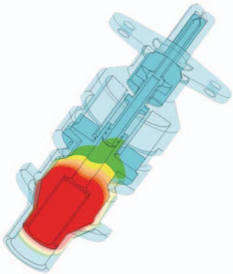
Fuel injector—The turbine engine fuel injector is part of a turbine engine used in road transport vehicles designed by an engineering firm. Shown is the steady-state heat transfer analysis performed in ALGOR to determine the temperature distribution from convection loads applied to the inner shaft and the outside surface of the entire assembly. Brick elements (not shown) were used in the model. (Courtesy of ALGOR, Inc.)
natural_image
Color-coded 3D thermal or stress simulation visualization of a cylindrical mechanical component (no text or symbols)
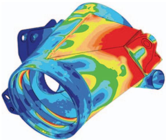
Housing model—The housing model made of ASTM A-572, grade 50 steel, is the rear-axle housing of a mining truck. A finite element analysis of the housing was necessary to determine why the housing failed in the field. The stress analysis performed using brick elements with torsional loads applied showed that the area around the padeye (shown in red color) was subjected to critical stresses, validating the visual inspection of the damaged part. The analysis was performed by a structural engineer working for the mining company. (Courtesy of ALGOR, Inc.)
natural_image
3D finite element mesh model of a mechanical component with color-coded stress or flow visualization (no text or symbols)
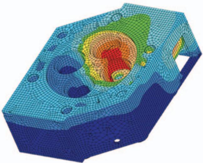
Cylinder head—The cylinder head model made of stainless steel AISI 410, is part of a prototype diesel engine that would provide reduced heat rejection and increased power density. Shown is the ALGOR steady-state heat transfer analysis (using brick elements) revealing the high temperatures of 1500 degrees F in red color at the interface between the two exhaust ports. These temperatures were then fed into the linear stress analyzer to obtain the thermal stresses ranging from 85 ksi to 200 ksi. The linear stress analysis confirmed the behavior that the engineers saw in the initial prototype tests. The highest thermal stresses coincided with the part of the cylinder head that had been leaking in the preliminary prototypes. (Courtesy of ALGOR, Inc.)
natural_image
3D simulation of a mechanical assembly with blue and yellow components, no visible text or symbols
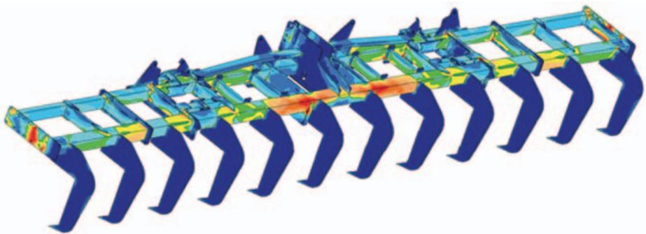
Subsoiler—The 12-row subsoiler used in agricultural equipment was designed to prepare 10 inch wide seed beds spaced 40 inches apart as commonly used in cotton production. One of these load conditions was simulating the shanks of the subsoiler pulling through 18 inches of hardpan soil. The ALGOR linear static stress analysis program was used to optimize the thickness, shape, and material of the frame, hitch and hinge components to reduce high stresses. The stress shown is the von Mises stress plot when the load is simulating the shanks pulling through approximately 18 inches of soil. From these results the designers can determine the parts that need to be made of stronger steel alloys. (Courtesy of ALGOR, Inc.)
natural_image
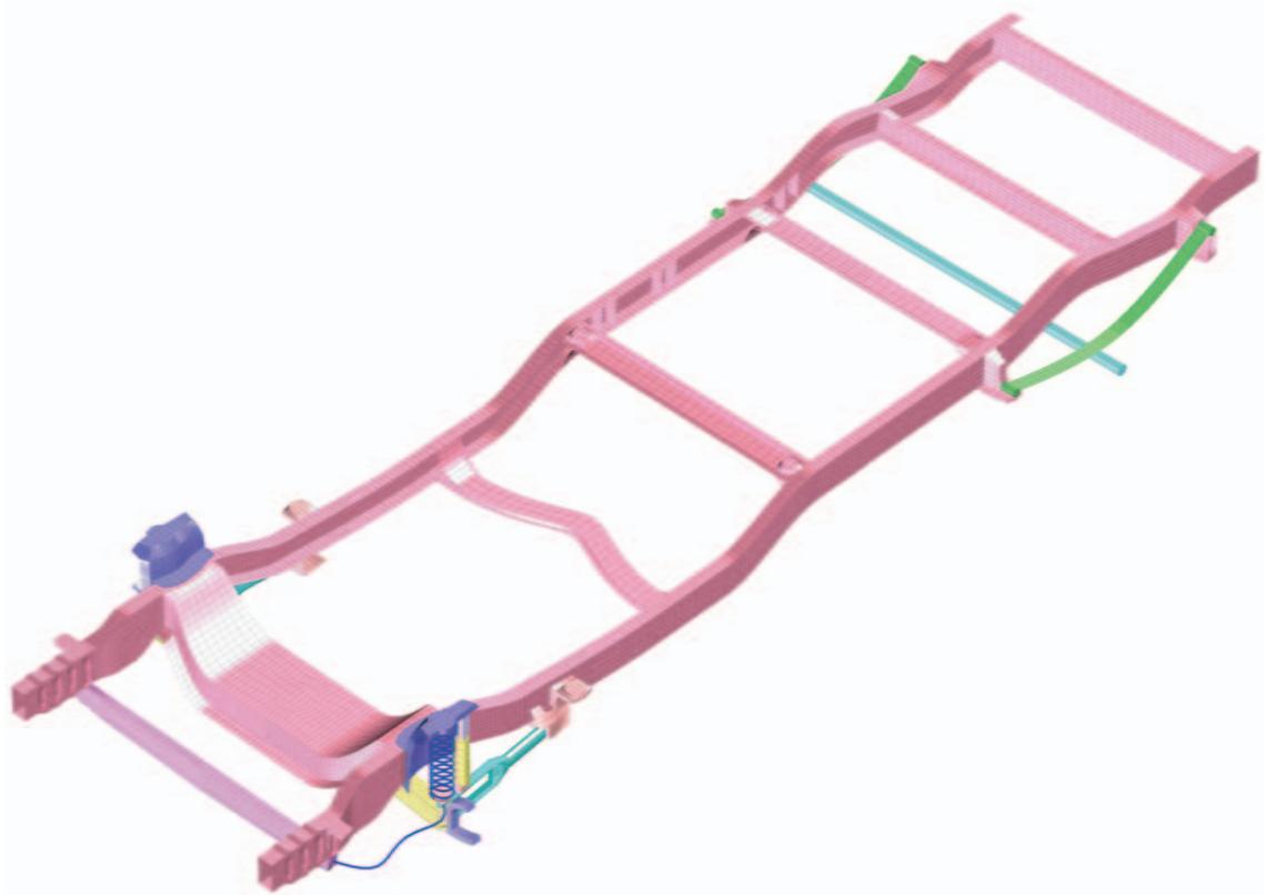
3D model of a pink structural frame with visible supports and components (no text or symbols)
Truck frame—Th e tru ck fra m e s h own is a fi n ite e l e m e nt m od e l m ad e of b ric k e l e m e nts. Th e stee l fra m e was d esig n ed to retrofit a t r u c k wi t h a n e l ect ri c m oto r wi t h batte ri es . (Co u rtesy of Tr u eG ri d 8.)
natural_image
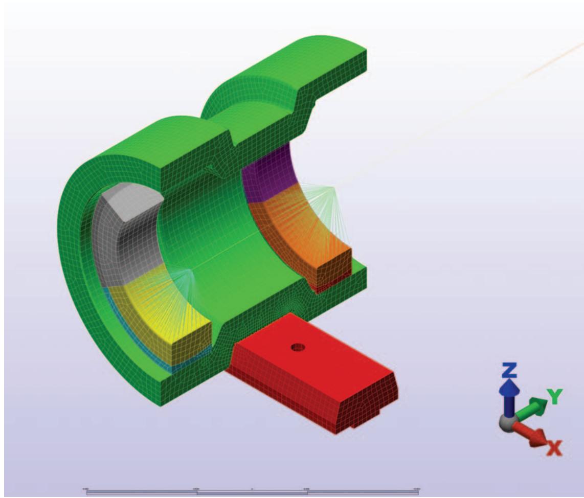
3D CAD model of a mechanical component with colored internal sections and a coordinate axis indicator (no text or symbols on the model itself)
Bearing housing—The steel bearing housing model is used to support one end of reel spool in the paper industry. A finite element model was created to study the deflection and stress in the bearing housing. The model consisted of beam elements to model the journal inside of the bearing, brick elements to model the bearings (multi-colored inside of the green colored bearing housing), bearing housing, and rail (orange color), universal joints to connect the journal to the bearing surface, surface contact pairs to represent the bearing-to-housing interface and housingto-rail interface. The model was created in Algor using FEMPRO. (Compliments of UW—Platteville students, Jason Fencl and David Stertz.)