text_image

s = +1 Node 1 s = 0 r s = -1 r = -1 r = 0 r = +1 x y

(a) 4 to 9 variable-number-nodes two-dimensional element Include only if node i is defined

		i=5	i=6	i=7	i=8	i=9
h1=	$\frac{1}{4}(1+r)(1+s)$	$-\frac{1}{2}h_{5}$			$-\frac{1}{2}h_{8}$	$-\frac{1}{4}h_{9}$
h2=	$\frac{1}{4}(1-r)(1+s)$	$-\frac{1}{2}h_{5}$	$-\frac{1}{2}h_{6}$			$-\frac{1}{4}h_{9}$
h3=	$\frac{1}{4}(1-r)(1-s)$		$-\frac{1}{2}h_{6}$	$-\frac{1}{2}h_{7}$		$-\frac{1}{4}h_{9}$
h4=	$\frac{1}{4}(1+r)(1-s)$			$-\frac{1}{2}h_{7}$	$-\frac{1}{2}h_{8}$	$-\frac{1}{4}h_{9}$
h5=	$\frac{1}{2}(1-r^{2})(1+s)$					$-\frac{1}{2}h_{9}$
h6=	$\frac{1}{2}(1-s^{2})(1-r)$					$-\frac{1}{2}h_{9}$
h7=	$\frac{1}{2}(1-r^{2})(1-s)$					$-\frac{1}{2}h_{9}$
h8=	$\frac{1}{2}(1-s^{2})(1+r)$					$-\frac{1}{2}h_{9}$
h9=	$(1-r^{2})(1-s^{2})$

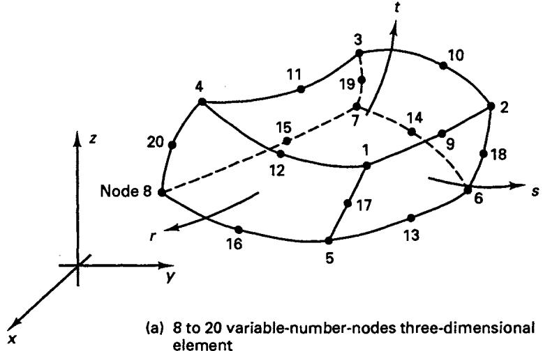
(b) Interpolation functions Figure 5.4 Interpolation functions of four to nine variable-number-nodes two-dimensional element 

text_image

(a) 8 to 20 variable-number-nodes three-dimensional element

Figure 5.5 Interpolation functions of eight to twenty variable-number-nodes three-dimensional element $$ h _ {1} = g _ {1} - \left(g _ {9} + g _ {1 2} + g _ {1 7}\right) / 2 \quad h _ {6} = g _ {6} - \left(g _ {1 3} + g _ {1 4} + g _ {1 8}\right) / 2 $$ $$ h _ {2} = g _ {2} - \left(g _ {9} + g _ {1 0} + g _ {1 8}\right) / 2 \quad h _ {7} = g _ {7} - \left(g _ {1 4} + g _ {1 5} + g _ {1 9}\right) / 2 $$ $$ h _ {3} = g _ {3} - \left(g _ {1 0} + g _ {1 1} + g _ {1 9}\right) / 2 \quad h _ {8} = g _ {8} - \left(g _ {1 5} + g _ {1 6} + g _ {2 0}\right) / 2 $$ $$ h _ {4} = g _ {4} - \left(g _ {1 1} + g _ {1 2} + g _ {2 0}\right) / 2 \quad h _ {j} = g _ {j} \text { for } j = 9, \dots , 2 0 $$ $$ h _ {5} = g _ {5} - \left(g _ {1 3} + g _ {1 6} + g _ {1 7}\right) / 2 $$ $g_{i} = 0$ if node $i$ is not included; otherwise, $$ g _ {i} = G (r, r _ {i}) G (s, s _ {i}) G (t, t _ {i}) $$ $$ G (\beta , \beta_ {i}) = \frac {1}{2} (1 + \beta_ {i} \beta) \quad \text { for } \beta_ {i} = \pm 1 $$ $$ G (\beta , \beta_ {i}) = (1 - \beta^ {2}) \quad \text { for } \beta_ {i} = 0 \quad ; \beta = r, s, t $$ (b) Interpolation functions Figure 5.5 (continued) The attractiveness of the elements in Figs. 5.3 to 5.5 lies in that the elements can have any number of nodes between the minimum and the maximum. Also, triangular elements can be formed (see Section 5.3.2). However, in general, to obtain maximum accuracy, the variable-number-nodes elements should be as nearly rectangular (in three-dimensional analysis, rectangular in each local plane) as possible and the noncorner nodes should, in general, be located at their natural coordinate positions; e.g., for the nine-node two-dimensional element the intermediate side nodes should, in general, be located at the midpoints between the corner nodes and the ninth node should be at the center of the element (for some exceptions see Section 5.3.2, and for more details on these observations, see Section 5.3.3). Considering the geometry of the two- and three-dimensional elements in Figs. 5.4 and 5.5 we note that by means of the coordinate interpolations in (5.18), the elements can have, without any difficulty, curved boundaries. This is an important advantage over the generalized coordinate finite element formulation. Another important advantage is the ease with which the element displacement functions can be constructed. In the isoparametric formulation the element displacements are interpolated in the same way as the geometry; i.e., we use $$ u = \sum_ {i = 1} ^ {q} h _ {i} u _ {i}; \quad v = \sum_ {i = 1} ^ {q} h _ {i} v _ {i}; \quad w = \sum_ {i = 1} ^ {q} h _ {i} w _ {i} \tag {5.19} $$ where u, v, and w are the local element displacements at any point of the element and $u_{i}$ , $v_{i}$ , and $w_{i}$ , $i = 1, \ldots, q$ , are the corresponding element displacements at its nodes. Therefore, it is assumed that to each nodal point coordinate necessary to describe the geometry of the element, there corresponds one nodal point displacement. $^{1}$ To be able to evaluate the stiffness matrix of an element, we need to calculate the strain-displacement transformation matrix. The element strains are obtained in terms of derivatives of element displacements with respect to the local coordinates. Because the element displacements are defined in the natural coordinate system using (5.19), we need to relate the x, y, z derivatives to the r, s, t derivatives, where we realize that (5.18) is of the form $$ x = f _ {1} (r, s, t); \quad y = f _ {2} (r, s, t); \quad z = f _ {3} (r, s, t) \tag {5.20} $$ where $f_{i}$ denotes “function of.” The inverse relationship is $$ r = f _ {4} (x, y, z); \quad s = f _ {5} (x, y, z); \quad t = f _ {6} (x, y, z) \tag {5.21} $$ We require the derivatives $\partial/\partial x$ , $\partial/\partial y$ , and $\partial/\partial z$ , and it seems natural to use the chain rule in the following form: $$ \frac {\partial}{\partial x} = \frac {\partial}{\partial r} \frac {\partial r}{\partial x} + \frac {\partial}{\partial s} \frac {\partial s}{\partial x} + \frac {\partial}{\partial t} \frac {\partial t}{\partial x} \tag {5.22} $$ with similar relationships for $\partial/\partial y$ and $\partial/\partial z$ . However, to evaluate $\partial/\partial x$ in (5.22), we need to calculate $\partial r/\partial x$ , $\partial s/\partial x$ , and $\partial t/\partial x$ , which means that the explicit inverse relationships in (5.21) would need to be evaluated. These inverse relationships are, in general, difficult to establish explicitly, and it is necessary to evaluate the required derivatives in the following way. Using the chain rule, we have $$ \left[ \begin{array}{l} \frac {\partial}{\partial r} \\ \frac {\partial}{\partial s} \\ \frac {\partial}{\partial t} \end{array} \right] = \left[ \begin{array}{l l l} \frac {\partial x}{\partial r} & \frac {\partial y}{\partial r} & \frac {\partial z}{\partial r} \\ \frac {\partial x}{\partial s} & \frac {\partial y}{\partial s} & \frac {\partial z}{\partial s} \\ \frac {\partial x}{\partial t} & \frac {\partial y}{\partial t} & \frac {\partial z}{\partial t} \end{array} \right] \left[ \begin{array}{l} \frac {\partial}{\partial x} \\ \frac {\partial}{\partial y} \\ \frac {\partial}{\partial z} \end{array} \right] \tag {5.23} $$ or, in matrix notation, $\frac{\partial}{\partial\mathbf{r}} = \mathbf{J}\frac{\partial}{\partial\mathbf{x}}$ (5.24) where J is the Jacobian operator relating the natural coordinate derivatives to the local coordinate derivatives. We should note that the Jacobian operator can easily be found using (5.18). We require $\partial/\partial x$ and use $$ \frac {\partial}{\partial \mathbf {x}} = \mathbf {J} ^ {- 1} \frac {\partial}{\partial \mathbf {r}} \tag {5.25} $$ which requires that the inverse of J exists. This inverse exists provided that there is a one-to-one (i.e., unique) correspondence between the natural and the local coordinates of the element, as expressed in (5.20) and (5.21). In most formulations the one-to-one correspondence between the coordinate systems (i.e., to each r, s, and t there corresponds only one x, y, and z) is obviously given, such as for the elements in Figs. 5.3 to 5.5. However, in cases where the element is much distorted or folds back upon itself, as in Fig. 5.6, the unique relation between the coordinate systems does not exist (see also Section 5.3.2 for singularities in the Jacobian transformation, Example 5.17). Using (5.19) and (5.25), we evaluate $\partial u / \partial x$ , $\partial u / \partial y$ , $\partial u / \partial z$ , $\partial v / \partial x$ , $\ldots$ , $\partial w / \partial z$ and can therefore construct the strain-displacement transformation matrix $\mathbf{B}$ , with $$ \epsilon = \mathbf {B} \hat {\mathbf {u}} \tag {5.26} $$  Figure 5.6 Elements with possible singular Jacobian where $\hat{u}$ is a vector listing the element nodal point displacements of (5.19), and we note that J affects the elements in B. The element stiffness matrix corresponding to the local element degrees of freedom is then $$ \mathbf {K} = \int_ {V} \mathbf {B} ^ {T} \mathbf {C} \mathbf {B} d V \tag {5.27} $$ We should note that the elements of B are functions of the natural coordinates r, s, and t. Therefore, the volume integration extends over the natural coordinate volume, and the volume differential dV need also be written in terms of the natural coordinates. In general, we have $$ d V = \det \mathbf {J} d r d s d t \tag {5.28} $$ where det J is the determinant of the Jacobian operator in (5.24) (see Exercise 5.6). An explicit evaluation of the volume integral in $(5.27)$ is, in general, not effective, particularly when higher-order interpolations are used or the element is distorted. Therefore, numerical integration is employed. Indeed, numerical integration must be regarded as an integral part of isoparametric element matrix evaluations. The details of the numerical integration procedures are described in Section 5.5, but the process can briefly be summarized as follows. First, we write $(5.27)$ in the form $$ \mathbf {K} = \int_ {V} \mathbf {F} d r d s d t \tag {5.29} $$ where $F = B^{T}CB$ det J and the integration is performed in the natural coordinate system of the element. As stated above, the elements of F depend on r, s, and t, but the detailed functional relationship is usually not calculated. Using numerical integration, the stiffness matrix is now evaluated as $$ \mathbf {K} = \sum_ {i, j, k} \alpha_ {i j k} \mathbf {F} _ {i j k} \tag {5.30} $$ where $F_{ijk}$ is the matrix F evaluated at the point $(r_{i}, s_{j}, t_{k})$ , and $\alpha_{ijk}$ is a given constant that depends on the values of $r_{i}, s_{j}$ , and $t_{k}$ . The sampling points $(r_{i}, s_{j}, t_{k})$ of the function and the corresponding weighting factors $\alpha_{ijk}$ are chosen to obtain maximum accuracy in the integration. Naturally, the integration accuracy can increase as the number of sampling points is increased. The purpose of this brief outline of the numerical integration procedure was to complete the description of the general isoparametric formulation. The relative simplicity of the formulation may already be noted. It is the simplicity of the element formulation and the efficiency with which the element matrices can actually be evaluated in a computer that has drawn much attention to the development of the isoparametric and related elements. The formulation of the element mass matrix and load vectors is now straightforward. Namely, writing the element displacements in the form $$ \mathbf {u} (r, s, t) = \mathbf {H} \hat {\mathbf {u}} \tag {5.31} $$ where $\mathbf{H}$ is a matrix of the interpolation functions, we have, as in (4.34) to (4.37), $$ \mathbf {M} = \int_ {V} \rho \mathbf {H} ^ {T} \mathbf {H} d V \tag {5.32} $$ $$ \mathbf {R} _ {B} = \int_ {V} \mathbf {H} ^ {T} \mathbf {f} ^ {B} d V \tag {5.33} $$ $$ \mathbf {R} _ {S} = \int_ {S} \mathbf {H} ^ {S ^ {T}} \mathbf {f} ^ {S} d S \tag {5.34} $$ $$ \mathbf {R} _ {I} = \int_ {V} \mathbf {B} ^ {T} \boldsymbol {\tau} ^ {I} d V \tag {5.35} $$ These matrices are evaluated using numerical integration, as indicated for the stiffness matrix K in (5.30). In the evaluation we need to use the appropriate function F. To calculate the body force vector $R_{B}$ we use $F = H^{T}f^{B}$ det J, for the surface force vector we use $F = H^{S^{T}}f^{S}$ det $J^{S}$ , for the initial stress load vector we use $F = B^{T}\tau^{I}$ det J, and for the mass matrix we have $F = \rho H^{T}H$ det J. This formulation was for one-, two-, or three-dimensional elements. We shall now consider some specific cases and demonstrate the details of the calculation of element matrices. EXAMPLE 5.2: Derive the displacement interpolation matrix H, strain-displacement interpolation matrix B, and Jacobian operator J for the three-node truss element shown in Fig. E5.2. 

text_image

r = -1 r = 0 r = +1 1 3 2 x₁ L/2 L/2 x, u

Figure E5.2 Truss element with node 3 at center of element The interpolation functions of the element were given in Fig. E5.1. Thus, we have $$ \mathbf {H} = \left[ - \frac {r}{2} (1 - r) \quad \frac {r}{2} (1 + r) \quad (1 - r ^ {2}) \right] \tag {a} $$ The strain-displacement matrix B is obtained by differentiation of H with respect to r and premultiplying the result by the inverse of the Jacobian operator, $$ \mathbf {B} = \mathbf {J} ^ {- 1} \left[ \left(- \frac {1}{2} + r\right) \quad \left(\frac {1}{2} + r\right) \quad - 2 r \right] \tag {b} $$ To evaluate J formally we use $$ x = - \frac {r}{2} (1 - r) x _ {1} + \frac {r}{2} (1 + r) \left(x _ {1} + L\right) + (1 - r ^ {2}) \left(x _ {1} + \frac {L}{2}\right) $$ hence, $x = x_{1} + \frac{L}{2} +\frac{L}{2} r$ (c) where we may note that because node 3 is at the center of the truss, x is interpolated linearly between nodes 1 and 2. The same result would be obtained using only nodes 1 and 2 for the geometry interpolation. Using now the relation in (c), we have $$ \mathbf {J} = \left[ \frac {L}{2} \right] \tag {d} $$ and $\mathbf{J}^{-1} = \left[\frac{2}{L}\right];\quad \operatorname *{det}\mathbf{J} = \frac{L}{2}$ With the relations in (a) to (d), we can now evaluate all finite element matrices and vectors given in (5.27) to (5.35). EXAMPLE 5.3: Establish the Jacobian operator J of the two-dimensional elements shown in Fig. E5.3.  Figure E5.3 Some two-dimensional elements The Jacobian operator is the same for the global X, Y and the local x, y coordinate systems. For convenience we therefore use the local coordinate systems. Substituting into (5.18) and (5.23) using the interpolation functions given in Fig. 5.4, we obtain for element 1: $$ x = 3 r; \quad y = 2 s $$ $$ \mathbf {J} = \left[ \begin{array}{l l} 3 & 0 \\ 0 & 2 \end{array} \right] $$ Similarly, for element 2, we have $$ \begin{array}{l} x = \frac {1}{4} \{(1 + r) (1 + s) [ 3 + 1 / (2 \sqrt {3}) ] + (1 - r) (1 + s) [ - (3 - 1 / (2 \sqrt {3})) ] \\ + (1 - r) (1 - s) \left[ - (3 + 1 / (2 \sqrt {3})) \right] + (1 + r) (1 - s) \left[ 3 - 1 / (2 \sqrt {3}) \right] \rbrace \\ y = \frac {1}{4} \left\{\left(1 + r\right) (1 + s) \left(\frac {1}{2}\right) + (1 - r) (1 + s) \left(\frac {1}{2}\right) + (1 - r) (1 - s) \left(- \frac {1}{2}\right) \right. \\ + (1 + r) (1 - s) \left(- \frac {1}{2}\right) \} \\ \end{array} $$ and hence, $$ \mathbf {J} = \left[ \begin{array}{c c} 3 & 0 \\ \frac {1}{2 \sqrt {3}} & \frac {1}{2} \end{array} \right] $$ Also, for element 3, $$ \begin{array}{l} x = \frac {1}{4} [ (1 + r) (1 + s) (1) + (1 - r) (1 + s) (- 1) + (1 - r) (1 - s) (- 1) \\ \left. + (1 + r) (1 - s) (+ 1) \right] \\ y = \frac {1}{4} [ (1 + r) (1 + s) (\frac {5}{4}) + (1 - r) (1 + s) (\frac {1}{4}) + (1 - r) (1 - s) (- \frac {3}{4}) \\ \left. + (1 + r) (1 - s) \left(- \frac {3}{4}\right) \right] \\ \end{array} $$ therefore, $$ \mathbf {J} = \frac {1}{4} \left[ \begin{array}{l l} 4 & (1 + s) \\ 0 & (3 + r) \end{array} \right] $$ We may recognize that the Jacobian operator of a $2 \times 2$ square element is the identity matrix, and that the entries in the operator J of a general element express the amount of distortion from that $2 \times 2$ square element. Since the distortion is constant at any point $(r, s)$ of elements 1 and 2, the operator J is constant for these elements. EXAMPLE 5.4: Establish the interpolation functions of the two-dimensional element shown in Fig. E5.4. 

text_image

2/3 cm 2/3 cm 2/3 cm 2 6 5 1 2 cm s r 3 4 7

(a) Figure E5.4 A seven-node element  Figure E5.4 (continued) The individual functions are obtained by combining the basic linear, parabolic, and cubic interpolations corresponding to the r and s directions. Thus, using the functions in Figure 5.3, we obtain $$ h _ {5} = \left[ \frac {1}{1 6} (- 2 7 r ^ {3} - 9 r ^ {2} + 2 7 r + 9) \right] \left[ \frac {1}{2} (1 + s) \right] $$ $$ h _ {6} = \left[ \left(1 - r ^ {2}\right) + \frac {1}{1 6} \left(2 7 r ^ {3} + 7 r ^ {2} - 2 7 r - 7\right) \right] \left[ \frac {1}{2} (1 + s) \right] $$ $$ h _ {2} = \left[ \frac {1}{2} (1 - r) - \frac {1}{2} (1 - r ^ {2}) + \frac {1}{1 6} (- 9 r ^ {3} + r ^ {2} + 9 r - 1) \right] \left[ \frac {1}{2} (1 + s) \right] $$ $$ h _ {3} = \frac {1}{4} (1 - r) (1 - s) $$ $$ h _ {7} = \frac {1}{2} (1 - s ^ {2}) (1 + r) $$ $$ h _ {4} = \frac {1}{4} (1 + r) (1 - s) - \frac {1}{2} h _ {7} $$ $$ h _ {1} = \frac {1}{4} (1 + r) (1 + s) - \frac {2}{3} h _ {5} - \frac {1}{3} h _ {6} - \frac {1}{2} h _ {7} $$ where $h_1$ is constructed as indicated in an oblique/aerial view in Fig. E5.4. EXAMPLE 5.5: Derive the expressions needed for the evaluation of the stiffness matrix of the isoparametric four-node finite element in Fig. E5.5. Assume plane stress or plane strain conditions. Using the interpolation function $h_{1}$ , $h_{2}$ , $h_{3}$ , and $h_{4}$ defined in Fig. 5.4, the coordinate interpolation given in (5.18) is, for this element, $$ x = \frac {1}{4} (1 + r) (1 + s) x _ {1} + \frac {1}{4} (1 - r) (1 + s) x _ {2} + \frac {1}{4} (1 - r) (1 - s) x _ {3} + \frac {1}{4} (1 + r) (1 - s) x _ {4} $$ $$ y = \frac {1}{4} (1 + r) (1 + s) y _ {1} + \frac {1}{4} (1 - r) (1 + s) y _ {2} + \frac {1}{4} (1 - r) (1 - s) y _ {3} + \frac {1}{4} (1 + r) (1 - s) y _ {4} $$ The displacement interpolation given in (5.19) is $$ u = \frac {1}{4} (1 + r) (1 + s) u _ {1} + \frac {1}{4} (1 - r) (1 + s) u _ {2} + \frac {1}{4} (1 - r) (1 - s) u _ {3} + \frac {1}{4} (1 + r) (1 - s) u _ {4} $$ $$ v = \frac {1}{4} (1 + r) (1 + s) v _ {1} + \frac {1}{4} (1 - r) (1 + s) v _ {2} + \frac {1}{4} (1 - r) (1 - s) v _ {3} + \frac {1}{4} (1 + r) (1 - s) v _ {4} $$ 

text_image

Node 1 s y, v r Node 2 Node 3 y4 x4 Node 4 x, u

Figure E5.5 Four-node two-dimensional element The element strains are given by $$ \boldsymbol {\epsilon} ^ {T} = \left[ \begin{array}{c c c} \epsilon_ {x x} & \epsilon_ {y y} & \gamma_ {x y} \end{array} \right] $$ where $\epsilon_{xx} = \frac{\partial u}{\partial x};\qquad \epsilon_{yy} = \frac{\partial v}{\partial y};\qquad \gamma_{xy} = \frac{\partial u}{\partial y} +\frac{\partial v}{\partial x}$ To evaluate the displacement derivatives, we need to evaluate (5.23): $$ \left[ \begin{array}{c} \frac {\partial}{\partial r} \\ \frac {\partial}{\partial s} \end{array} \right] = \left[ \begin{array}{c c} \frac {\partial x}{\partial r} & \frac {\partial y}{\partial r} \\ \frac {\partial x}{\partial s} & \frac {\partial y}{\partial s} \end{array} \right] \left[ \begin{array}{c} \frac {\partial}{\partial x} \\ \frac {\partial}{\partial y} \end{array} \right] \quad \text { or } \quad \frac {\partial}{\partial \mathbf {r}} = \mathbf {J} \frac {\partial}{\partial \mathbf {x}} $$ where $\frac{\partial x}{\partial r} = \frac{1}{4} (1 + s)x_1 - \frac{1}{4} (1 + s)x_2 - \frac{1}{4} (1 - s)x_3 + \frac{1}{4} (1 - s)x_4$ $$ \frac {\partial x}{\partial s} = \frac {1}{4} (1 + r) x _ {1} + \frac {1}{4} (1 - r) x _ {2} - \frac {1}{4} (1 - r) x _ {3} - \frac {1}{4} (1 + r) x _ {4} $$ $$ \frac {\partial y}{\partial r} = \frac {1}{4} (1 + s) y _ {1} - \frac {1}{4} (1 + s) y _ {2} - \frac {1}{4} (1 - s) y _ {3} + \frac {1}{4} (1 - s) y _ {4} $$ $$ \frac {\partial y}{\partial s} = \frac {1}{4} (1 + r) y _ {1} + \frac {1}{4} (1 - r) y _ {2} - \frac {1}{4} (1 - r) y _ {3} - \frac {1}{4} (1 + r) y _ {4} $$ Therefore, for any value $r$ and $s, -1 \leq r \leq +1$ and $-1 \leq s \leq +1$ , we can form the Jacobian operator $\mathbf{J}$ by using the expressions shown for $\partial x / \partial r$ , $\partial x / \partial s$ , and $\partial y / \partial r$ , $\partial y / \partial s$ . Assume that we evaluate $\mathbf{J}$ at $r = r_i$ and $s = s_j$ and denote the operator by $\mathbf{J}_{ij}$ and its determinant by $\det \mathbf{J}_{ij}$ . Then we have $$ \left[ \begin{array}{c}\frac{\partial}{\partial x}\\ \frac{\partial}{\partial y} \end{array} \right]_{\substack{\text{at} r = r_{i}\\ s = s_{j}}} = \mathbf{J}_{ij}^{-1}\left[ \begin{array}{c}\frac{\partial}{\partial r}\\ \frac{\partial}{\partial s} \end{array} \right]_{\substack{\text{at} r = r_{i}\\ s = s_{j}}} $$ To evaluate the element strains we use $$ \frac {\partial u}{\partial r} = \frac {1}{4} (1 + s) u _ {1} - \frac {1}{4} (1 + s) u _ {2} - \frac {1}{4} (1 - s) u _ {3} + \frac {1}{4} (1 - s) u _ {4} $$ $$ \frac {\partial u}{\partial s} = \frac {1}{4} (1 + r) u _ {1} + \frac {1}{4} (1 - r) u _ {2} - \frac {1}{4} (1 - r) u _ {3} - \frac {1}{4} (1 + r) u _ {4} $$ $$ \frac {\partial v}{\partial r} = \frac {1}{4} (1 + s) v _ {1} - \frac {1}{4} (1 + s) v _ {2} - \frac {1}{4} (1 - s) v _ {3} + \frac {1}{4} (1 - s) v _ {4} $$ $$ \frac {\partial v}{\partial s} = \frac {1}{4} (1 + r) v _ {1} + \frac {1}{4} (1 - r) v _ {2} - \frac {1}{4} (1 - r) v _ {3} - \frac {1}{4} (1 + r) v _ {4} $$ Therefore, $$ \left[ \begin{array}{l} \frac {\partial u}{\partial x} \\ \frac {\partial u}{\partial y} \end{array} \right] _ {\text {at} r = r _ {i}} = \frac {1}{4} \mathbf {J} _ {i j} ^ {- 1} \left[ \begin{array}{c c c c c c c c c} 1 + s _ {j} & 0 & - (1 + s _ {j}) & 0 & - (1 - s _ {j}) & 0 & 1 - s _ {j} & 0 \\ 1 + r _ {i} & 0 & 1 - r _ {i} & 0 & - (1 - r _ {i}) & 0 & - (1 + r _ {i}) & 0 \end{array} \right] \hat {\mathbf {u}} \tag {a} $$ and $$ \left[ \begin{array}{l} \frac {\partial v}{\partial x} \\ \frac {\partial v}{\partial y} \end{array} \right] _ {\text {at} r = r _ {i}} = \frac {1}{4} \mathbf {J} _ {i j} ^ {- 1} \left[ \begin{array}{l l l l l l l l l} 0 & 1 + s _ {j} & 0 & - (1 + s _ {j}) & 0 & - (1 - s _ {j}) & 0 & 1 - s _ {j} \\ 0 & 1 + r _ {i} & 0 & 1 - r _ {i} & 0 & - (1 - r _ {i}) & 0 & - (1 + r _ {i}) \end{array} \right] \hat {\mathbf {u}} \tag {b} $$ where $\hat{\mathbf{u}}^T = [u_1 \quad v_1 \quad u_2 \quad v_2 \quad u_3 \quad v_3 \quad u_4 \quad v_4]$ Evaluating the relations in (a) and (b), we can establish the strain-displacement transformation matrix at the point $(r_{i}, s_{j})$ ; i.e., we obtain $$ \mathbf {e} _ {i j} = \mathbf {B} _ {i j} \hat {\mathbf {u}} $$ where the subscripts $i$ and $j$ indicate that the strain-displacement transformation is evaluated at the point $(r_i, s_j)$ . For example, if $x = r$ , $y = s$ (i.e., the stiffness matrix of a square element is required that has side lengths equal to 2), the Jacobian operator is the identity matrix, and hence $$ B _ {i j} = \frac {1}{4} \left[ \begin{array}{c c c c c c c c} 1 + s _ {j} & 0 & - (1 + s _ {j}) & 0 & - (1 - s _ {j}) & 0 & 1 - s _ {j} & 0 \\ 0 & 1 + r _ {i} & 0 & 1 - r _ {i} & 0 & - (1 - r _ {i}) & 0 & - (1 + r _ {i}) \\ 1 + r _ {i} & 1 + s _ {j} & 1 - r _ {i} & - (1 + s _ {j}) & - (1 - r _ {i}) & - (1 - s _ {j}) & - (1 + r _ {i}) & 1 - s _ {j} \end{array} \right] $$ The matrix $\mathbf{F}_{ij}$ in (5.30) is now simply $$ \mathbf {F} _ {i j} = \mathbf {B} _ {i j} ^ {T} \mathbf {C B} _ {i j} \det \mathbf {J} _ {i j} $$ where the material property matrix C is given in Table 4.3. In the case of plane stress or plane strain conditions, we integrate in the r, s plane and assume that the function F is constant through the thickness of the element. The stiffness matrix of the element is therefore $$ \mathbf {K} = \sum_ {i, j} t _ {i j} \alpha_ {i j} \mathbf {F} _ {i j} $$