Input file template ```txt *HEADING ... *PSD-DEFINITION, NAME=name, TYPE=type Data lines to define a frequency function (or PSD function for moving noise) ** *STEP *FREQUENCY Data line to control eigenvalue extraction *BOUNDARY Data lines to assign degrees of freedom to the primary base *END STEP *STEP *RANDOM RESPONSE Data line to specify frequency range of interest *SELECT EIGENMODES Data lines to define the applicable mode ranges *MODAL DAMPING Data line to define modal damping *CORRELATION, PSD=name, TYPE=type Data lines to specify correlation for various excitation load cases (n, p) *DLOAD Data lines to define distributed loads *CLOAD, LOAD CASE=n Data lines to define concentrated loads in load case n *CONNECTOR LOAD, LOAD CASE=m Data lines to define connector loads in load case m *BASE MOTION, DOF=dof, LOAD CASE=p Data lines to define base motion p *END STEP ``` # 6.4 Steady-state transport analysis • “Steady-state transport analysis,” Section 6.4.1 # 6.4.1 STEADY-STATE TRANSPORT ANALYSIS # Product: Abaqus/Standard # References • “Defining an analysis,” Section 6.1.2 • “Symmetric model generation,” Section 10.4.1 • \*STEADY STATE TRANSPORT • \*SYMMETRIC MODEL GENERATION • \*MOTION • \*TRANSPORT VELOCITY • \*ACOUSTIC FLOW VELOCITY # Overview A steady-state transport analysis: • allows for steady-state rolling and sliding solutions including frictional effects and inertia effects; • allows for steady-state solutions to be obtained directly or by using a quasi-steady-state (pass-bypass) technique; • is used to model the interaction between a deformable rolling object and one or more flat, convex, or concave surfaces; • is based on a specialized analysis capability where the rigid body motion is described in a spatial or Eulerian manner and the deformation in a material or Lagrangian manner; • allows for one element set in a model to be described in an Eulerian manner while the rest of the elements in the model are treated in a classical Lagrangian manner; • can be preceded by a static stress analysis or followed by a natural frequency extraction or a complex eigenvalue extraction step; • uses regular stress/displacement elements and special steady-state rolling and sliding contact pairs; • is currently available only for three-dimensional analysis with an axisymmetric geometry or a periodic geometry; and • allows rate-independent, rate-dependent, or history-dependent material behavior. # Steady-state transport analysis It is cumbersome to model rolling and sliding contact, such as a tire rolling along a rigid surface or a disc rotating relative to a brake assembly, using a traditional Lagrangian formulation since the frame of reference in which motion is described is attached to the material. An observer in this reference frame views even steady-state rolling as a time-dependent process since each point undergoes a repeated history of deformation. Such an analysis is computationally expensive since a transient analysis must be performed and fine meshing is required along the entire surface of the cylinder. The steady-state transport analysis capability in Abaqus/Standard uses a reference frame that is attached to the axle of the rotating cylinder. An observer in this frame sees the cylinder as points that are not moving, although the material of which the cylinder is made is moving through those points. This removes the explicit time dependence from the problem—the observer sees a fixed point anywhere, with material moving through it. Thus, the finite element mesh describing the cylinder in this frame of reference does not undergo the large rigid body spinning motion. This means that a fine mesh is required only near the contact zone. This description can be viewed as a mixed Lagrangian/Eulerian method, where rigid body rotation is described in a spatial or Eulerian manner, and deformation, which is now measured relative to the rotating rigid body, is described in a material or Lagrangian manner. It is this kinematic description that converts the steady-state moving contact problem into a purely spatially dependent simulation. The steady-state rolling and sliding analysis capability provides solutions that include frictional effects, inertia effects, and material convection for most rate-independent, rate-dependent, and historydependent material models. The theory is described in detail in “Steady-state transport analysis,” Section 2.7.1 of the Abaqus Theory Guide. Input File Usage: \*STEADY STATE TRANSPORT # Pass-by-pass analysis technique By default, the steady-state transport analysis procedure in Abaqus/Standard solves for a steady-state rolling and sliding solution directly as a series of increments, with iterations to obtain equilibrium within each increment. The solution in each increment is a steady-state solution corresponding to the loads acting on the structure at that instant. The steady-state transport analysis procedure also provides an alternative technique to obtain a quasi-steady-state rolling and sliding solution as a series of increments, with iterations to obtain equilibrium within each increment. However, the solution in each increment is usually not a steady-state solution corresponding to the loads acting on the structure at that instant. A steady-state solution is generally obtained in several increments, with each increment corresponding to a loading pass through the structure. Each loading pass through the structure can have a different magnitude. The pass-by-pass analysis technique is relevant only when used with plasticity/creep models. It has no effect on a viscoelastic material model. Input File Usage: \*STEADY STATE TRANSPORT, PASS BY PASS # Unstable problems Local instabilities (e.g., surface wrinkling, material instability, or local buckling), can occur in a steadystate transport analysis. Abaqus/Standard offers the option to stabilize this class of problems by applying damping throughout the model in such a way that the viscous forces introduced are sufficiently large to prevent instantaneous buckling or collapse but small enough not to affect the behavior significantly while the problem is stable. The available automatic stabilization schemes are described in detail in “Automatic stabilization of unstable problems” in “Solving nonlinear problems,” Section 7.1.1. # Defining the model A steady-state transport analysis requires the definition of streamlines. The streamlines are the trajectories that the material follows during transport through the mesh. To meet this requirement, the mesh must be generated using the symmetric model generation capability, which is described in detail in “Symmetric model generation,” Section 10.4.1. The three-dimensional model can be created either by revolving an axisymmetric model about its axis of revolution or by revolving a single three-dimensional repetitive sector about its axis of symmetry. # Revolving an axisymmetric cross-section to create a three-dimensional model You can generate a three-dimensional mesh by revolving a two-dimensional cross-section about a symmetry axis, so that the streamlines follow the mesh lines. In this case the symmetric model generation capability requires a two-dimensional cross-section of the body as a starting point. The cross-section, which must be discretized with axisymmetric finite elements, is defined in a separate input file. A data check analysis must be performed to write the model information to a restart file. The restart file is read in a subsequent run, and a three-dimensional model is generated by Abaqus/Standard by revolving the cross-section about the symmetry axis, starting at a reference plane. Both the symmetry axis and reference plane of the new three-dimensional model can be oriented in any direction in the global coordinate system. The symmetry axis also defines the axis of the spinning body. A nonuniform discretization in the circumferential direction can be specified to allow a finer mesh in the contact region than elsewhere in the model. Input File Usage: \*SYMMETRIC MODEL GENERATION, REVOLVE # Revolving a single three-dimensional sector to create a periodic model Alternatively, you can generate a periodic three-dimensional mesh by revolving a single three-dimensional sector about its axis of symmetry. To accurately account for the material convection when the streamline integration is performed, the segment angle for the repetitive three-dimensional sector must be chosen small enough. In this case the symmetric model generation capability requires a single three-dimensional sector as a starting point. The original three-dimensional sector is defined in a separate input file. A data check analysis must be performed to write the model information to a restart file. The restart file is read in a subsequent run, and a three-dimensional periodic model is generated by Abaqus/Standard by revolving the original three-dimensional sector about the symmetry axis. Both the symmetry axis and the original three-dimensional repetitive sector can be oriented in any direction in the global coordinate system. The symmetry axis also defines the axis of the spinning body. There is no restriction that the meshes on the two symmetry surfaces of the repetitive sector match in any way. If the surface meshes on either side of the original sector are not matched completely, constraints will be generated automatically to couple the opposing neighboring surfaces when revolving the original sector to create a periodic model. Input File Usage: $\boldsymbol { * } \mathrm { S Y M M E T R I C ~ M O D E L ~ G E N E R A T I O N } , \mathrm { P E R I O D I C }$ # Identifying the elements being treated in an Eulerian manner By default, the rigid body motion in the whole model will be described in a spatial or Eulerian manner. In some cases you may want only part of the model to be treated with the Eulerian method while the rest should be treated with the classical Lagrangian method. One typical example is a disc brake where the disc itself can be treated with the Eulerian method while the brake assembly (brake pads and caliper) is treated with the Lagrangian method. In this case you can specify the name of an element set for which the rigid body motion will be described in an Eulerian manner. The elements that are not included in the element set will be treated with the classical Lagrangian method. Only one Eulerian element set can be specified in the whole model. In a new steady-state transport step or upon restart (see “Restarting an analysis,” Section 9.1.1) you can respecify a set of elements to be treated with the Eulerian method even after it has previously been treated with the Lagrangian method and vice versa. Elements treated with the Eulerian method and elements treated with the Lagrangian method cannot be mixed along a streamline. 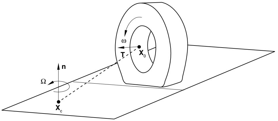Input File Usage: \*STEADY STATE TRANSPORT, ELSET=name # Defining reference frame motions The deformable and rigid bodies can each be defined in their own moving reference frame in a steadystate rolling and sliding analysis. The motion of these reference frames can be defined quite generally and provides modeling of a spinning deformable body traveling along a straight line, or “cornering” or “precessing” around an axis such as shown in Figure 6.4.1–1. It is also possible to define reference frame motions for rigid bodies, including translations and rotations. The rigid body can be flat, convex, or concave, which allows for modeling of a deformable body in contact with a rotating drum, such as a tire rolling on a drum, or for modeling a tire mounted on a rigid rim. 

text_image

n Ω Xc ω T X0

Figure 6.4.1–1 Constant cornering example showing conventions for defining reference frame motions. When defining different reference frame motions for bodies that interact, you must make sure that the interactions are indeed steady. For example, for a planar rigid surface the relative reference frame motion must be tangential to the rigid surface, and for a body of revolution the relative reference frame motion must be rotation around its axis. Convergence difficulties will persist if the interactions are not steady. # Spinning motion The spinning motion of the deformable body around its own axis is described by a user-specified angular velocity, (see Figure 6.4.1–1). This angular velocity defines the transport of material through the mesh; you define the magnitude of the spinning rotation, . The axis of revolution is the symmetry axis used for generating the mesh as described in “Defining the model.” The transport velocity must be defined for all nodes on the spinning body. The magnitude of the angular velocity can also be defined with user subroutine UMOTION. The transport velocity can also be applied to a rigid body based on a three-dimensional surface of revolution. In that case the velocity is applied to the rigid body reference node to describe the transport of the (rigid) material relative to the reference node. Abaqus/Standard assumes that the rigid body spins around the axis of revolution of the rigid body. This option can, for example, be applied to the rigid body representing the rim on which a tire is mounted. Abaqus/Standard will automatically update the position and orientation of the rotation axis to the current configuration in a large-displacement analysis, such as in the case where a prescribed load applied to the reference node of a rotating rigid drum maintains the contact pressure between the tire and drum or the case where a camber angle is applied to the axle of the deformable body. Input File Usage: Use either of the following options: \*TRANSPORT VELOCITY \*TRANSPORT VELOCITY, USER # Defining a reference frame for translational or rotational motion The rotating deformable body is also associated with a reference frame. This reference frame can either translate or rotate with respect to the fixed global reference frame. Similarly, each rigid body must be defined in a reference frame that is either fixed, translates, or rotates. For example, to associate straight line travel at ground velocity, , with a spinning deformable body, the deformable body can be defined in a reference frame translating at velocity and the rigid surface can be defined in a fixed reference frame. Alternatively, the deformable body can be defined in a reference frame that does not translate and the rigid body can be defined in a frame translating at velocity . Another example is a deformable body precessing along a circular path such as shown in Figure 6.4.1–1. In such a case a rotating frame is associated with the deformable body that defines the precession axis and angular velocity, while the rigid body is defined in a fixed reference frame. All components of the reference frame motion are zero unless otherwise specified; components of the reference frame motion cannot be treated as unknowns to be determined by the simulation. You can apply a specified motion of the reference frame to all nodes of the deformable body or to the reference node of a rigid body. A translating reference frame is defined by specifying the components of the velocity vector, . A rotating reference frame is defined by specifying the magnitude of an angular rotation velocity, , and the position and orientation of the axis of rotation in the current configuration. The position and orientation of the axis are applied at the beginning of the step and remain fixed during the step.

Input File Usage:

Use the following option to define the motion of a translating reference frame: *MOTION, TRANSLATIONUse the following option to define the motion of a rotating reference frame: *MOTION, ROTATION

# Contact conditions Abaqus/Standard provides contact between a rigid surface and deformable body moving with different velocities, such as contact between a rolling tire and the ground, as well as contact between surfaces moving with the same velocity, such as the contact between the bead and rim in a tire analysis. Abaqus/Standard also provides contact between two deformable bodies moving with the same velocity, such as the contact between the tread blocks on a tire surface, as well as contact between two deformable bodies moving with different velocities, such as the contact between a disc and brake assembly. # Contact between a rigid surface and a deformable body moving with different velocities The rigid surface can be either an analytical surface or made from rigid elements. When the master and slave surfaces move with different velocities, you will normally select to use a Coulomb friction law that assumes that slip occurs if the frictional stress $$ \tau_ {e q} = \sqrt {\tau_ {1} ^ {2} + \tau_ {2} ^ {2}} $$ is equal to the critical stress $\tau _ { c r i t } = \mu p$ , where $\tau _ { 1 }$ and $\tau _ { 2 }$ are the shear stresses on the contact plane, $\mu$ is the friction coefficient, and $\pmb { p }$ is the contact pressure. No slip occurs when $\tau _ { e q } < \tau _ { c r i t }$ . For steady-state transport the condition of no slip is approximated in Abaqus/Standard by stiff “viscous” behavior $$ \tau_ {\alpha} = \kappa_ {s} \dot {\gamma} _ {\alpha}, $$ where $\dot { \gamma } _ { \alpha }$ are the tangential slip velocities that depend on deformation along a streamline and $$ \kappa_ {s} = \frac {\mu p}{2 F _ {f} \omega R} $$ is the “stick viscosity,” R is the radius of the cylinder, and $F _ { f }$ is a user-defined slip tolerance for which the default is 0.005. Using a larger slip tolerance makes convergence of the solution more rapid at the expense of solution accuracy. Using a smaller slip tolerance imposes the “no relative motion” constraint more accurately but may slow convergence. The default value provides a conservative balance between efficiency and accuracy for rolling contact problems. Since this frictional model used for steady-state rolling is different from the frictional models used with other analysis procedures in Abaqus/Standard, discontinuities may arise in the solutions between a steady-state transport analysis and any other analysis procedure, such as a static footprint analysis. To ensure a smooth transition in the solution, it is recommended that all analysis steps prior to a steady-