text_image
ŷ, v̂
w
m̂(0)
L
m̂(L)
x̂
V̂(0)
V̂(L)
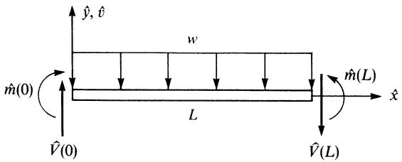
Figure 4–36 Beam element with shear forces, moments, and a distributed load
text_image
V̂(L)
V̂(0)
V̂(L)
V̂(0)
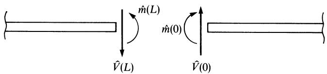
Figure 4–37 Shear forces and moments acting on adjacent elements meeting at a node
Note that when element matrices are assembled, two shear forces and two moments from adjacent elements contribute to the concentrated force and concentrated moment at the node common to the adjacent elements as shown in Figure 4–37. These concentrated shear forces $\hat { V } ( 0 ) - \hat { V } ( L )$ and moments $\hat { m } ( L ) - \hat { m } ( 0 )$ are often zero; that is, $\hat { V } ( 0 ) = \hat { V } ( L )$ and $\hat { m } ( L ) = \hat { m } ( 0 )$ occur except when a concentrated nodal force or moment exists at the node. In the actual computations, we handle the expressions given by Eq. (4.8.9) by including them as concentrated nodal values making up the matrix fPg.
# References
[1] Gere, J. M., Mechanics of Materials, 5th ed., Brooks/Cole Publishers, Pacific Grove, CA, 2001.
[2] Hsieh, Y. Y., Elementary Theory of Structures, 2nd ed., Prentice-Hall, Englewood Cliffs, NJ, 1982.
[3] Fraeijes de Veubeke, B., ‘‘Upper and Lower Bounds in Matrix Structural Analysis,’’ Matrix Methods of Structural Analysis, AGAR Dograph 72, B. Fraeijes de Veubeke, ed., Macmillan, New York, 1964.
[4] Juvinall, R. C., and Marshek, K. M., Fundamentals of Machine Component Design, 4th. ed., John Wiley & Sons, New York, 2006.
[5] Przemieneicki, J. S., Theory of Matrix Structural Analysis, McGraw-Hill, New York, 1968.
[6] McGuire, W., and Gallagher, R. H., Matrix Structural Analysis, John Wiley & Sons, New York, 1979.
[7] Severn, R. T., ‘‘Inclusion of Shear Deflection in the Stiffness Matrix for a Beam Element’’, Journal of Strain Analysis, Vol. 5, No. 4, 1970, pp. 239–241.
[8] Narayanaswami, R., and Adelman, H. M., ‘‘Inclusion of Transverse Shear Deformation in Finite Element Displacement Formulations’’, AIAA Journal, Vol. 12, No. 11, 1974, 1613–1614.
[9] Timoshenko, S., Vibration Problems in Engineering, 3rd. ed., Van Nostrand Reinhold Company, 1955.
[10] Clark, S. K., Dynamics of Continous Elements, Prentice Hall, 1972.
[11] Algor Interactive Systems, 260 Alpha Dr., Pittsburgh, PA 15238.
# Problems
4.1 Use Eqs. (4.1.7) to plot the shape functions $N _ { 1 }$ and $N _ { 3 }$ and the derivatives $( d N _ { 2 } / d \hat { x } )$ and $( d N _ { 4 } / d \hat { x } )$ , which represent the shapes (variations) of the slopes $\hat { \phi } _ { 1 }$ and $\hat { \phi } _ { 2 }$ over the length of the beam element.
4.2 Derive the element stiffness matrix for the beam element in Figure 4–1 if the rotational degrees of freedom are assumed positive clockwise instead of counterclockwise. Compare the two different nodal sign conventions and discuss. Compare the resulting stiffness matrix to Eq. (4.1.14).
Solve all problems using the finite element stiffness method.
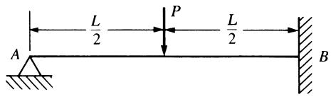
4.3 For the beam shown in Figure P4–3, determine the rotation at pin support A and the rotation and displacement under the load P. Determine the reactions. Draw the shear force and bending moment diagrams. Let EI be constant throughout the beam.
text_image
L/2
P
L/2
A
B
Figure P4–3
text_image
P
A
L
B
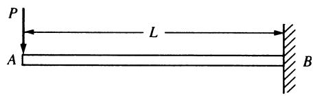
Figure P4–4
4.4 For the cantilever beam subjected to the free-end load P shown in Figure P4–4, determine the maximum deflection and the reactions. Let EI be constant throughout the beam.
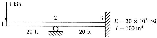
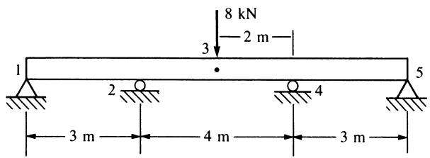
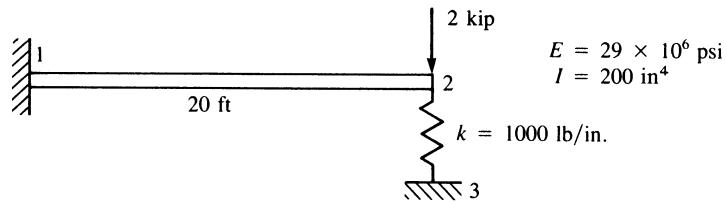
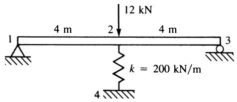
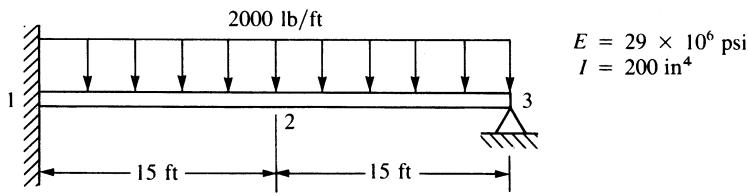
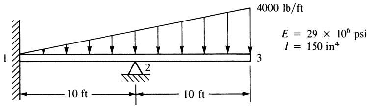
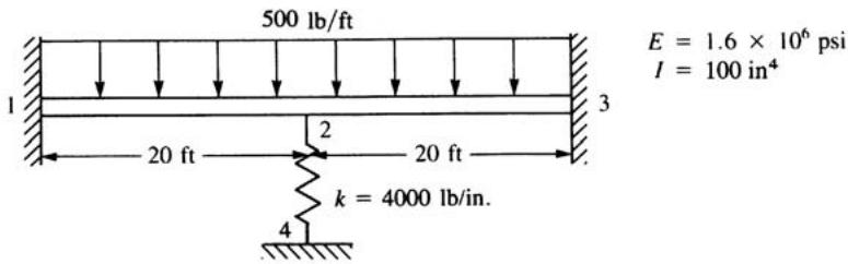
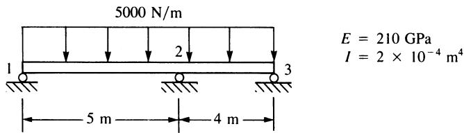
4.5–4.11 For the beams shown in Figures P4–5—P4–11, determine the displacements and the slopes at the nodes, the forces in each element, and the reactions. Also, draw the shear force and bending moment diagrams.
text_image
1 kip
1
2
3
E = 30 × 10⁶ psi
I = 100 in⁴
20 ft
20 ft
Figure P4–5
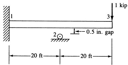
text_image
1 kip
1
3
0.5 in. gap
2
20 ft
20 ft
$$
E = 3 0 \times 1 0 ^ {6} \mathrm{psi}
$$
$$
I = 1 0 0 \mathrm{in} ^ {4}
$$
(Compare answers with P4-5.)
Figure P4–6
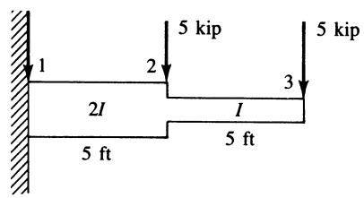
text_image
1
2
2l
5 ft
5 kip
3
5 kip
I
5 ft
$$
E = 3 0 \times 1 0 ^ {6} \mathrm{psi}
$$
$$
I = 2 0 0 \mathrm{in} ^ {4}
$$
Figure P4–7
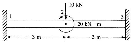
text_image
10 kN
2
20 kN · m
3
3 m
3 m
$$
E = 2 1 0 \mathrm{GPa}
$$
$$
I = 4 \times 1 0 ^ {- 4} \mathrm{m} ^ {4}
$$
Figure P4–8
text_image
8 kN
— 2 m
3
1
2
4
5
3 m
4 m
3 m
$$
E = 7 0 \mathrm{GPa}
$$
$$
I = 1 \times 1 0 ^ {- 4} \mathrm{m} ^ {4}
$$
Figure P4–9
text_image
1
20 ft
2 kip
2
k = 1000 lb/in.
3
E = 29 × 10⁶ psi
I = 200 in⁴
Figure P4–10
text_image
12 kN
4 m 2 4 m
k = 200 kN/m
1 3
4
$$
\begin{array}{r l} E & = 7 0 \mathrm{GPa} \\ I & = 2 \times 1 0 ^ {- 4} \mathrm{m} ^ {4} \end{array}
$$
Figure P4–11
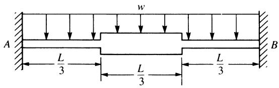
4.12 For the fixed-fixed beam subjected to the uniform load w shown in Figure P4–12, determine the midspan deflection and the reactions. Draw the shear force and bending moment diagrams. The middle section of the beam has a bending stiffness of 2EI; the other sections have bending stiffnesses of EI .
text_image
w
A
L/3
L/3
L/3
B
Figure P4–12
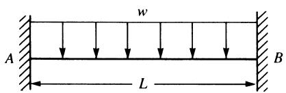
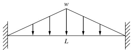
4.13 Determine the midspan deflection and the reactions and draw the shear force and bending moment diagrams for the fixed-fixed beam subjected to uniformly distributed load w shown in Figure P4–13. Assume EI constant throughout the beam. Compare your answers with the classical solution (that is, with the appropriate equivalent joint forces given in Appendix D).
text_image
w
A
L
B
Figure P4–13
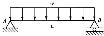
text_image
w
A L B
O
Figure P4–14
4.14 Determine the midspan deflection and the reactions and draw the shear force and bending moment diagrams for the simply supported beam subjected to the uniformly distributed load w shown in Figure P4–14. Assume EI constant throughout the beam.
4.15 For the beam loaded as shown in Figure P4–15, determine the free-end deflection and the reactions and draw the shear force and bending moment diagrams. Assume EI constant throughout the beam.
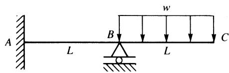
text_image
A
L
B
w
L
C
Figure P4–15
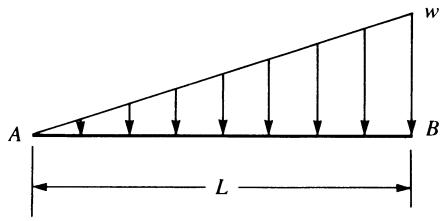
text_image
A
L
B
w
Figure P4–16
4.16 Using the concept of work equivalence, determine the nodal forces and moments (called equivalent nodal forces) used to replace the linearly varying distributed load shown in Figure P4–16.
4.17 For the beam shown in Figure 4–17, determine the displacement and slope at the center and the reactions. The load is symmetrical with respect to the center of the beam. Assume EI constant throughout the beam.
text_image
w
L
Figure P4–17
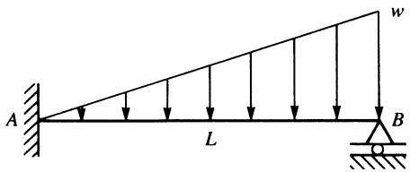
4.18 For the beam subjected to the linearly varying line load w shown in Figure P4–18, determine the right-end rotation and the reactions. Assume EI constant throughout the beam.
text_image
A
L
B
w
Figure P4–18
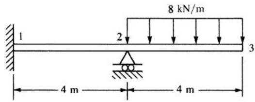
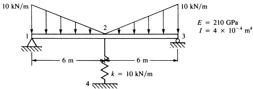
4.19–4.24 For the beams shown in Figures P4–19—P4–24, determine the nodal displacements and slopes, the forces in each element, and the reactions.
text_image
8 kN/m
1
2
3
4 m
4 m
$$
E = 7 0 \mathrm{GPa}
$$
$$
I = 3 \times 1 0 ^ {- 4} \mathrm{m} ^ {4}
$$
Figure P4–19
text_image
10 kN/m
10 kN/m
E = 210 GPa
I = 4 × 10⁻⁴ m⁴
1
2
3
6 m
6 m
k = 10 kN/m
4
Figure P4–20
text_image
2000 lb/ft
E = 29 × 10⁶ psi
I = 200 in⁴
1
2
3
15 ft
15 ft
Figure P4–21
text_image
4000 lb/ft
E = 29 × 10⁶ psi
I = 150 in⁴
1
2
3
10 ft
10 ft
Figure P4–22
text_image
500 lb/ft
E = 1.6 × 10⁶ psi
I = 100 in⁴
1
2
3
20 ft
20 ft
k = 4000 lb/in.
4
Figure P4–23
text_image
5000 N/m
E = 210 GPa
I = 2 × 10⁻⁴ m⁴
1
2
3
5 m
4 m
Figure P4–24
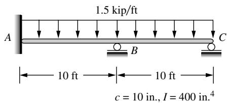
4.25–31 For the beams shown in Figures P4–25—P4–30, determine the maximum deflection and maximum bending stress. Let E ¼ 200 GPa or $3 0 \times 1 0 ^ { 6 }$ psi for all beams as appropriate for the rest of the units in the problem. Let c be the half-depth of each beam.
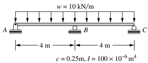
text_image
w = 10 kN/m
A B C
4 m 4 m
c = 0.25m, I = 100 × 10⁻⁶ m⁴
Figure P4–25
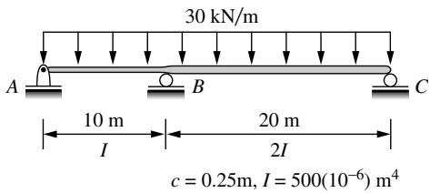
text_image
30 kN/m
A B C
10 m 20 m
I 2I
c = 0.25m, I = 500(10^-6) m^4
Figure P4–26
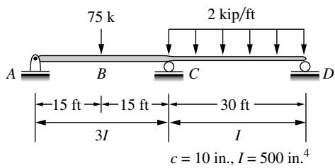
text_image
75 k
2 kip/ft
A B C D
15 ft 15 ft 30 ft
3I I
c = 10 in., I = 500 in.⁴
Figure P4–27
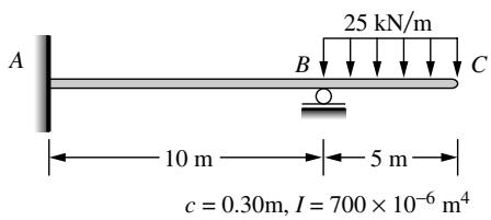
text_image
A
25 kN/m
B
C
10 m
5 m
c = 0.30m, I = 700 × 10⁻⁶ m⁴
Figure P4–28
text_image
1.5 kip/ft
A
B
C
10 ft
10 ft
c = 10 in., I = 400 in.⁴
Figure P4–29
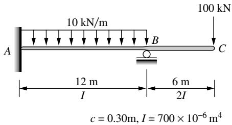
text_image
10 kN/m
100 kN
A
B
C
12 m
I
6 m
2I
c = 0.30m, I = 700 × 10⁻⁶ m⁴
Figure P4–30
For the beam design problems shown in Figures P4–31 through P4–36, determine the size of beam to support the loads shown, based on requirements listed next to each beam.

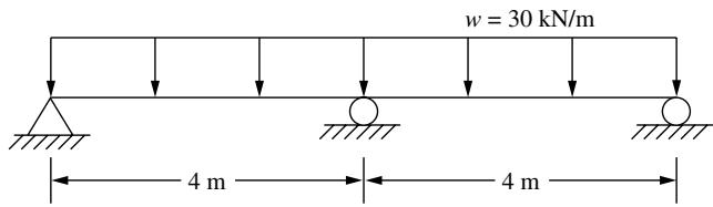
4.31 Design a beam of ASTM A36 steel with allowable bending stress of 160 MPa to support the load shown in Figure P4–31. Assume a standard wide flange beam from Appendix F or some other source can be used.
text_image
w = 30 kN/m
4 m
4 m
Figure P4–31


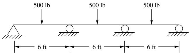
4.32 Select a standard steel pipe from Appendix F to support the load shown. The allowable bending stress must not exceed 24 ksi, and the allowable deflection must not exceed $\mathrm { L } / 3 6 0$ of any span.
text_image
500 lb
500 lb
500 lb
6 ft
6 ft
6 ft
Figure P4–32

4.33 Select a rectangular structural tube from Appendix F to support the loads shown for the beam in Figure P4–33. The allowable bending stress should not exceed 24 ksi.
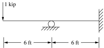
text_image
1 kip
6 ft
6 ft
Figure P4–33

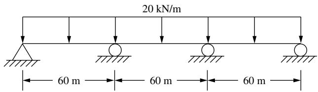
4.34 Select a standard W section from Appendix F or some other source to support the loads shown for the beam in Figure P4–34. The bending stress must not exceed 160 MPa.
text_image
20 kN/m
60 m 60 m 60 m
Figure P4–34

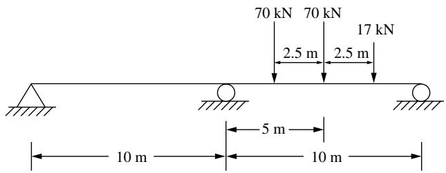
4.35 For the beam shown in Figure P4–35, determine a suitable sized W section from Appendix F or from another suitable source such that the bending stress does not exceed 150 MPa and the maximum deflection does not exceed $\mathrm { L } / 3 6 0$ of any span.
text_image
70 kN 70 kN 17 kN
2.5 m 2.5 m
10 m 5 m 10 m
Figure P4–35

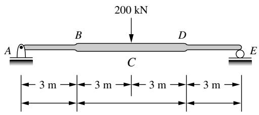
4.36 For the stepped shaft shown in Figure P4–36, determine a solid circular cross section for each section shown such that the bending stress does not exceed 160 MPa and the maximum deflection does not exceed L/360 of the span.
text_image
200 kN
A B C D E
3 m 3 m 3 m 3 m
Figure P4–36
4.37 For the beam shown in Figure P4–37 subjected to the concentrated load P and distributed load w, determine the midspan displacement and the reactions. Let EI be constant throughout the beam.
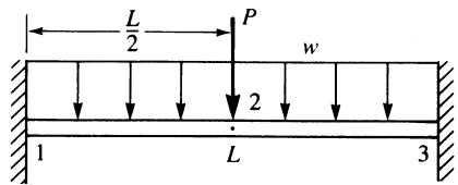
text_image
L/2
P
w
2
1
L
3
Figure P4–37
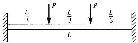
text_image
L/3
P
L/3
P
L/3
L
Figure P4–38
4.38 For the beam shown in Figure P4–38 subjected to the two concentrated loads P, determine the deflection at the midspan. Use the equivalent load replacement method. Let EI be constant throughout the beam.
4.39 For the beam shown in Figure P4–39 subjected to the concentrated load P and the linearly varying line load w, determine the free-end deflection and rotation and the reactions. Use the equivalent load replacement method. Let EI be constant throughout the beam.
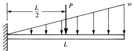
text_image
L/2
P
w
L
Figure P4–39
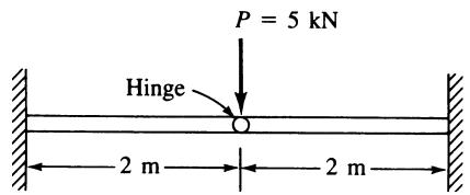
text_image
P = 5 kN
Hinge
2 m
2 m
Figure P4–40
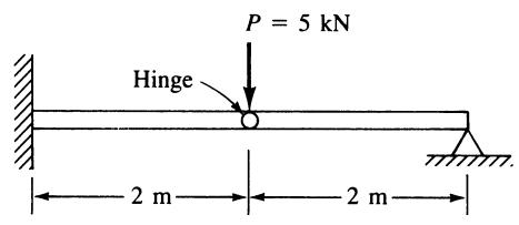
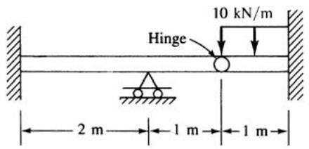
4.40–42 For the beams shown in Figures P4–40—P4–42, with internal hinge, determine the deflection at the hinge. Let E ¼ 210 GPa and $I = 2 \times 1 0 ^ { - 4 } ~ \mathrm { m } ^ { 4 }$ .
text_image
P = 5 kN
Hinge
2 m
2 m
Figure P4–41
text_image
10 kN/m
Hinge
2 m
1 m
1 m
Figure P4–42
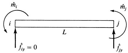
4.43 Derive the stiffness matrix for a beam element with a nodal linkage—that is, the shear is 0 at node i, but the usual shear and moment resistance are present at node j (see Figure P4–43).
text_image
m̂_i
i
L
j
m̂_j
f̂_iy = 0
f̂_jy
Figure P4–43
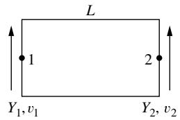
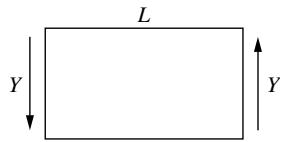
4.44 Develop the stiffness matrix for a fictitious pure shear panel element (Figure P4–44) in terms of the shear modulus, G the shear web area, $A _ { W }$ , and the length, L. Notice the Y and v are the shear force and transverse displacement at each node, respectively.
$\mathrm { G i v e n ~ ~ \xi ~ 1 \ / } \ \tau = G _ { \gamma } , \quad \mathrm { 2 ) } \ Y = \tau _ { \mathrm { A w } } , \quad \mathrm { 3 ) } \ Y _ { \mathrm { 1 } } + Y _ { \mathrm { 2 } } = 0 , \quad \mathrm { 4 ) } \ \gamma = \frac { v _ { \mathrm { 2 } } - v _ { \mathrm { 1 } } } { \cal L }$
text_image
L
1
2
Y₁,v₁
Y₂,v₂
Positive node force sign convention
text_image
L
Y
Y
Element in equilibrium (neglect moments)
Figure P4–44
4.45 Explicitly evaluate $\pi _ { p }$ of Eq. (4.7.15); then differentiate $\pi _ { p }$ with respect to $\hat { d } _ { 1 y } , \hat { \phi } _ { 1 } , \hat { d } _ { 2 y }$ , and $\hat { \phi } _ { 2 }$ and set each of these equations to zero (that is, minimize $\pi _ { p } )$ to obtain the four element equations for the beam element. Then express these equations in matrix form.
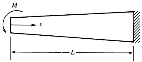
4.46 Determine the free-end deflection for the tapered beam shown in Figure P4–46. Here $I ( x ) = I _ { 0 } ( 1 + n x / L )$ where $I _ { 0 }$ is the moment of inertia at $x = 0 .$ . Compare the exact beam theory solution with a two-element finite element solution for $n = 2$ .
text_image
M
x
L
Figure P4–46
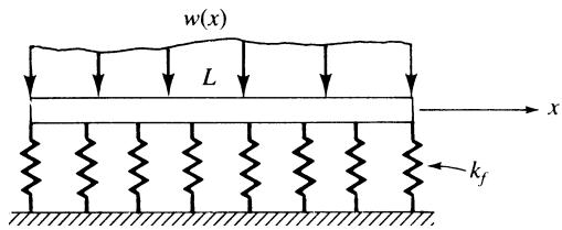
text_image
w(x)
L
x
k_f
Figure P4–47