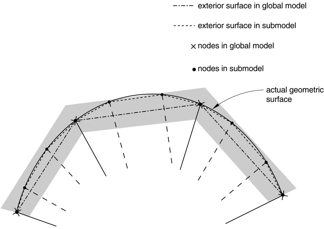
text_image

exterior surface in global model exterior surface in submodel × nodes in global model ● nodes in submodel actual geometric surface

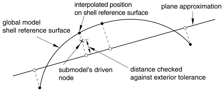
Figure 10.2.2–6 The exterior tolerance in solid-to-solid submodeling. through the node on the submodel with the reference surface of the shell in the global model. The direction of the line is normal to a flat surface approximation to each shell element. The normal to the flat surface is the average of the normals at the nodes of the shell element. The distance checked against the specified exterior tolerance is shown in Figure 10.2.2–7. # The exterior tolerance in shell-to-solid submodeling For shell-to-solid submodeling Abaqus uses two kinds of tolerances to determine the relationship between the submodel and the global model. First, the closest point on the shell reference surface of the global model is determined. This point, the “image node,” is shown in Figure 10.2.2–8. The user-specified exterior tolerance is used to check if the image node lies within the domain of the global model. Then the distance, , between the driven node and its image is checked; if the distance is less than half the value of the specified shell thickness plus the exterior tolerance, it is accepted. This check is only approximate if the global model has varying shell thickness or if the shell reference surface is offset from the midsurface. 

flowchart

```mermaid graph TD A["global model shell reference surface"] --> B["submodel's driven node"] B --> C["interpolated position on shell reference surface"] C --> D["plane approximation"] D --> E["distance checked against exterior tolerance"] E --> A ```

Figure 10.2.2–7 Flat surface approximation in shell-to-shell submodeling. 

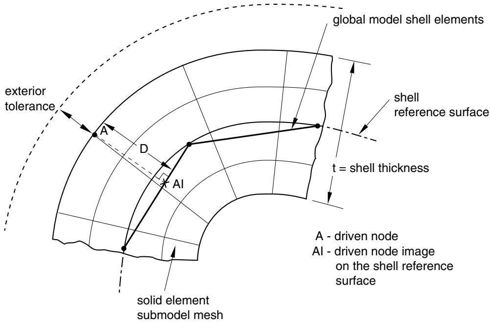
text_image

global model shell elements shell reference surface t = shell thickness exterior tolerance A D AI solid element submodel mesh A - driven node AI - driven node image on the shell reference surface

Figure 10.2.2–8 The exterior tolerance in shell-to-solid submodeling. # Permitting driven nodes to be excluded from submodeling In some cases (such as when your submodel geometry is more detailed than the global model in regions near a free surface) you may specify driven nodes that Abaqus will find, even when accounting for the search tolerance, to be outside the region of the global model elements. By default, these cases result in an error message. In solid-to-solid submodeling you can, however, specify that Abaqus ignore driven nodes that cannot be found. Use this option with caution and always evaluate the list of nodes that are labeled as not found. Most cases where Abaqus finds driven nodes to lie outside the global model reflect a modeling error and use of the intersection only option may lead to incorrect results in these cases. # Input File Usage: Use the following option to specify that Abaqus ignore driven nodes that cannot be found in the global model elements: \*SUBMODEL, INTERSECTION ONLY list of nodes or node set labels The driven nodes ignored through the use of the INTERSECTION ONLY parameter are then ignored in all subsequent submodel boundary condition references. # Defining the driven variables in the submodel The actual driven variables are defined in any step as a submodel boundary condition. The boundary conditions are “driven variables” obtained from the results or output database file of the global analysis. The degrees of freedom on the driven nodes of the submodel must exist at the forcing nodes of the global model. In a problem involving an acoustic fluid submodel driven by a structural global model, for example, acoustic interface elements should be created on the submodel’s driven boundary with the structure. For solid-to-solid and shell-to-shell submodeling specify the individual degrees of freedom to be driven. In most cases all components of the solution variables (displacements, rotations, temperatures, etc.) at these nodes are driven by the global solution, although you may choose to drive only some components at any of the driven nodes. For shell-to-solid submodeling the driven degrees of freedom are chosen automatically based on a user-specified zone around the shell reference surface, as explained later. Abaqus/Explicit does not admit jumps in displacement and rotation boundary conditions (see “Prescribed displacement” in “Boundary conditions in Abaqus/Standard and Abaqus/Explicit,” Section 34.3.1); any jumps in the driven displacements and rotations will be ignored. It is not recommended to have all the variables at all the nodes in the submodel driven by the global solution. For acoustic-to-structure submodeling, the loads due to acoustic pressure acting at the driven nodes of the submodel are activated by specifying pressure (degree of freedom 8) along with the driven node set. Only one submodel boundary condition can be specified in each step of the analysis. # Input File Usage: \*BOUNDARY, SUBMODEL # Abaqus/CAE Usage: Load module: Create Boundary Condition: choose Other for the Category and Submodel for the Types for Selected Step: select region: Degrees of freedom: degrees of freedom # Specifying the step number from the global analysis You specify the step of the global model history that is to be used for the driven variables in the current submodel analysis step. When the global solution is obtained from the results file, the zero increment is included if it was requested in the global analysis (see “Output,” Section 4.1.1). In a general analysis step or a direct-solution steady-state dynamic analysis step, Abaqus calculates the amplitudes for the driven variables as functions of time or frequency from the results of the global model. Input File Usage: \*BOUNDARY, SUBMODEL, STEP=step Abaqus/CAE Usage: Load module: Create Boundary Condition: choose Other for the Category and Submodel for the Types for Selected Step: select region: Global step number: step Scaling the global time period to the submodel time period The global analysis and submodel analysis can have different time steps. You can scale the time variable of the driven nodes from the global analysis to the step time of the submodel analysis. This technique is useful when the analyses are static or quasi-static in nature; the use of this technique in dynamic analyses with significant inertial effects is not recommended. If the same step time is used in both the global model and the submodel, the time scale has no effect. The time scale cannot be specified in frequency domain analyses or in linear perturbation steps. Abaqus will determine the values that the driven variables will follow throughout the step in the submodel analysis by using the points in time at which the global solution results or output database file was written. When the time variable of the driven nodes of the global analysis is scaled and if the step time is different from the submodel step time, the points in time of the driven variables are scaled to the submodel step time. Input File Usage: \*BOUNDARY, SUBMODEL, STEP=step, TIMESCALE Abaqus/CAE Usage: Load module: Create Boundary Condition: choose Other for the Category and Submodel for the Types for Selected Step: select region: Scale time period of global step to time period of submodel step Scaling the magnitude of driven variables For displacement-based submodeling the magnitude values of driven variables are obtained by multiplying the displacement history as obtained from the global analysis by a scaling parameter. You can scale the driven variables by setting the scaling parameter in the definition of the submodel boundary conditions. This technique is useful in scaling the submodel boundary conditions in a multiple-step analysis without rerunning the global model. It can be used in Abaqus/Standard and Abaqus/Explicit for the same-to-same and shell-to-solid cases except for acoustic-to-structure submodeling. Input File Usage: \*BOUNDARY, SUBMODEL, STEP=step, SCALE=scalarValue Abaqus/CAE Usage: Load module: Create Boundary Condition: choose Other for the Category and Submodel for the Types for Selected Step: select region: Scale: scale # Modifying the set of driven variables You can modify the submodel boundary condition to add new variables to the list of driven variables, you can remove variables from the driven variable set, and you can reintroduce them later (see “Boundary conditions in Abaqus/Standard and Abaqus/Explicit,” Section 34.3.1). New nodes cannot be added to the total set of driven nodes defined for the submodel; this set of driven nodes is a fixed part of the model definition. 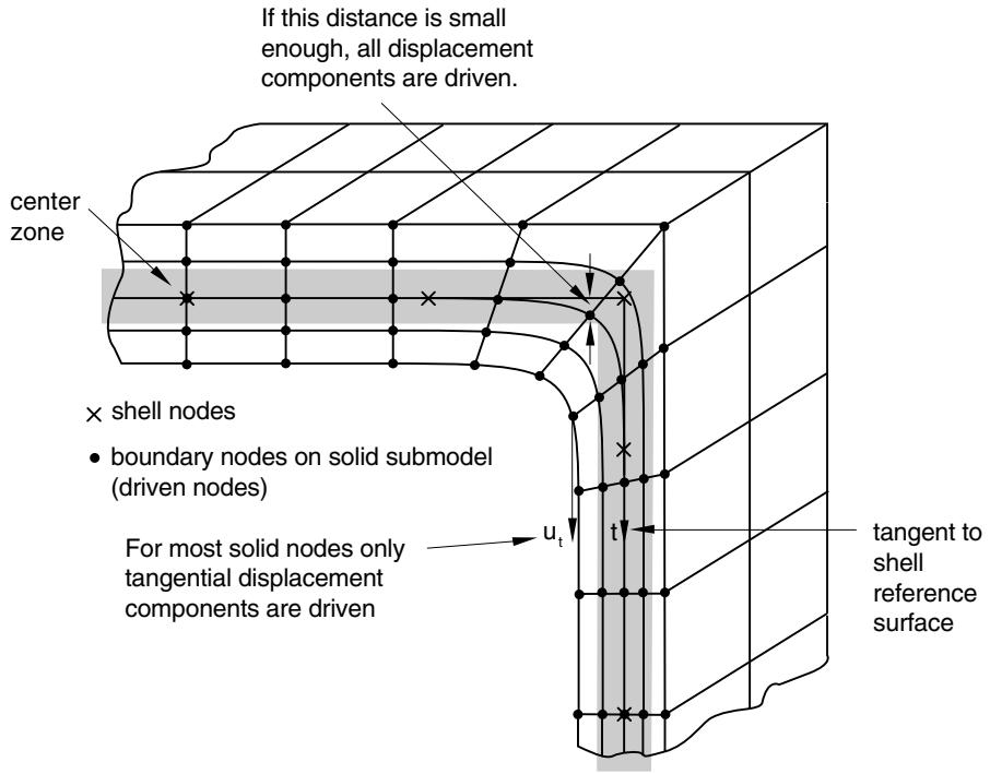Input File Usage: Use one of the following options: \*BOUNDARY, SUBMODEL, OP=MOD \*BOUNDARY, SUBMODEL, OP=NEW Abaqus/CAE Usage: Load module: boundary condition editor: Degrees of freedom # Automatically selecting the driven variables in shell-to-solid submodeling For shell-to-solid submodeling the driven degrees of freedom at the driven nodes are chosen automatically, depending on the distance between the driven node and the global model shell reference surface. All displacement components are driven at nodes that lie on the reference surface or within a “center zone,” as shown in Figure 10.2.2–9. The size of the center zone is specified as part of the submodel boundary condition definition, as described below. For nodes that lie further away from the reference surface, only the displacement components parallel to the shell reference surface are driven. At least one layer of nodes in the submodel must be within the center zone; if no nodes are found this close to the reference surface, Abaqus issues an error message. # Specifying the size of the center zone in shell-to-solid submodeling The center zone method of prescribing driven variables usually provides a reasonable transfer of the plane stress assumption in the shell model. The width of this zone around the reference surface where all displacement components are driven may be different for various driven nodes or node sets. If you do not provide values for the center zone size, a default value of 10% of the maximum of the specified shell thicknesses is assumed. For complicated geometries it can be advantageous to assign a different center zone size to different nodes or node sets. You can view the driven nodes lying inside and outside the center zone in Abaqus/CAE by displaying the model boundary conditions (View→ODB Display Options) in the Visualization module. Input File Usage: \*BOUNDARY, SUBMODEL, STEP=step nodes, center zone size Abaqus/CAE Usage: Load module: Create Boundary Condition: choose Other for the Category and Submodel for the Types for Selected Step: select region: Center zone size: center zone size # Transferring transverse shear stresses in shell-to-solid submodeling Usually it is enough for the layer of nodes closest to the shell reference surface to lie inside the center zone. If a very fine solid mesh is used in the thickness direction and substantial transverse shear stresses 

text_image

If this distance is small enough, all displacement components are driven. center zone × shell nodes • boundary nodes on solid submodel (driven nodes) For most solid nodes only tangential displacement components are driven u_t t tangent to shell reference surface

Figure 10.2.2–9 Center zone choice in shell-to-solid submodeling. are transferred, it may be necessary to make the center zone size large enough that multiple layers of nodes lie inside the zone. However, if the transverse shear stresses at the submodel boundary are high and the submodel is highly refined in the thickness direction, high local stresses may develop since the shear force at the submodel boundary is transferred only at the driven nodes within the center zone. High transverse shear stresses occur only in regions where bending moments vary rapidly; it is better not to locate the submodel boundary in such regions. It is best to locate the submodel boundary in areas of low transverse shear stress in the global model. # Special considerations There are several special considerations that are worth noting. # Specifying the shell thickness in shell-to-shell submodeling For shell-to-shell submodeling the shell thickness generally is not changed between the models. You can specify different shell thicknesses if, for example, a local thickness change is being investigated; however, Abaqus does not check the validity of these differences. 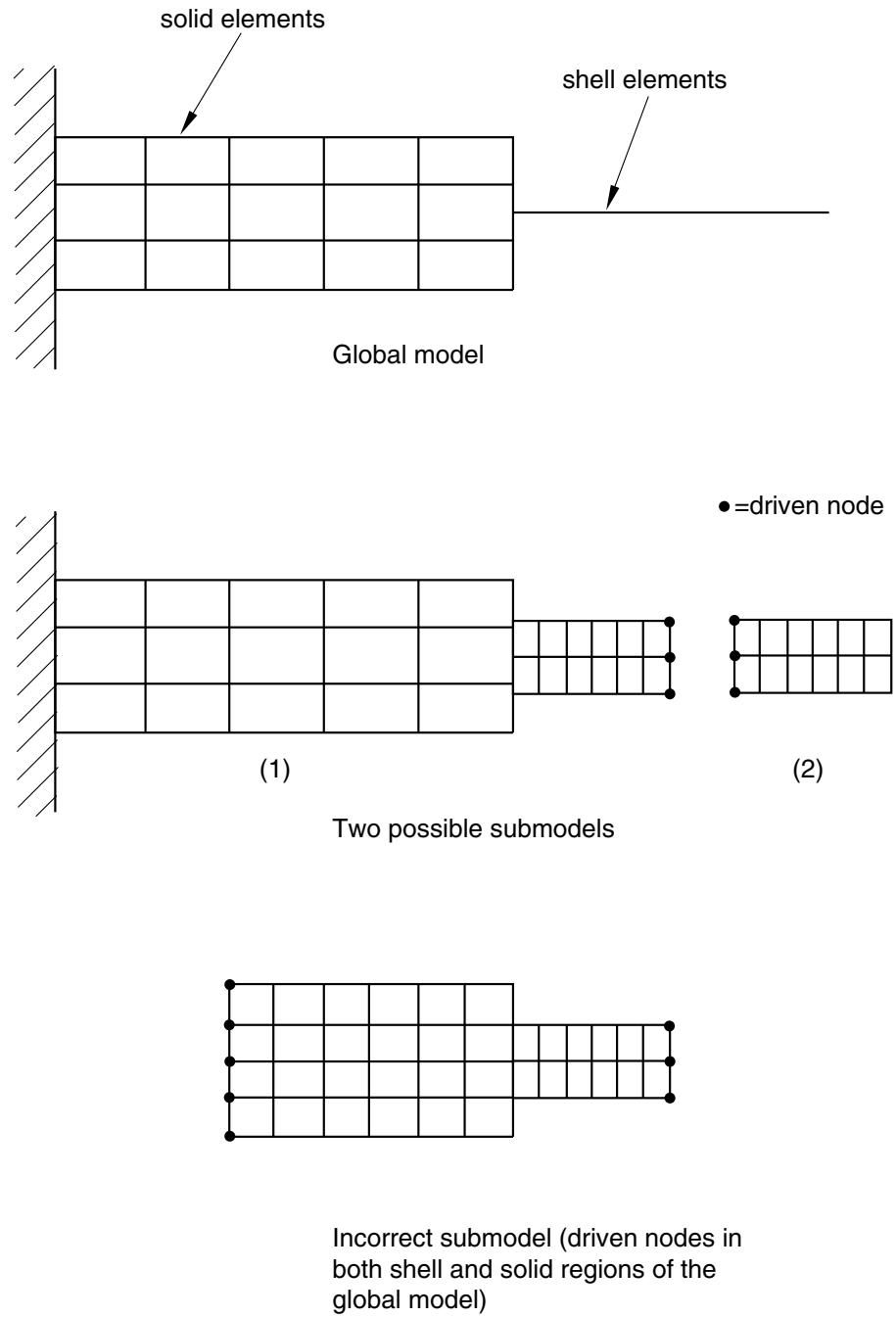# Limitations in shell-to-solid submodeling The following limitations and special cases apply to the shell-to-solid capability: • The global model can contain both solid and shell elements; however, when the shell-to-solid capability is used, all driven nodes must lie within shell elements in the global model. If the driven boundary lies at the border between a solid and a shell region, the driven nodes must be moved a small distance away from the solid region (see Figure 10.2.2–10). 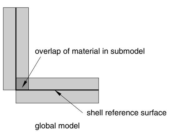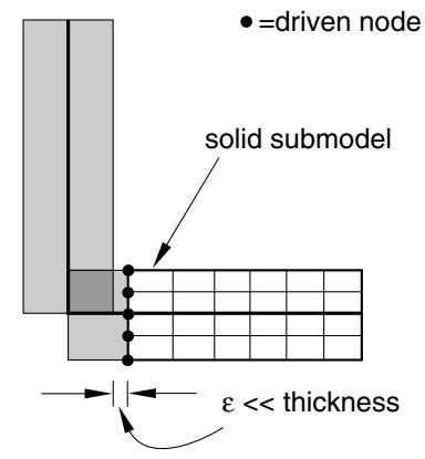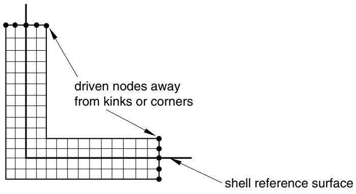Corners or kinks may exist in global models made of shell elements. At such corners or kinks the shell elements only approximate the distribution of the material away from the midsurface of the shell (see Figure 10.2.2–11). Because of such approximations, it is not possible to drive a submodel correctly if the driven nodes of the submodel lie within a shell thickness from a corner or a kink. If necessary, use the approach shown in Figure 10.2.2–11. A better approach is to include the corner or kink as part of the submodel and drive it from nodes well away from corners or kinks since they are a source of stress concentration and high stress gradients (see Figure 10.2.2–12). • Temperature degrees of freedom cannot be driven in shell-to-solid submodeling. # Alternative to shell-to-solid submodeling An alternative to shell-to-solid submodeling is the surface-based shell-to-solid coupling capability discussed in “Shell-to-solid coupling,” Section 35.3.3. # Procedures Neither the coupled thermal-electrical procedure nor any of the mode-based dynamics procedures can be used on the submodel level. In addition, submodeling cannot be used in conjunction with symmetric model generation or symmetric results transfer. Adaptive meshes should not be used in the global model. However, they can be used in the submodel analysis; Abaqus will always treat the driven nodes in the submodel as Lagrangian nodes. Both general (possibly nonlinear) and linear perturbation steps can be used in submodeling (see “General and linear perturbation procedures,” Section 6.1.3, for a discussion of general and linear perturbation steps). # Submodeling in dynamic procedures The submodeling capability can be used in the dynamic procedures using explicit integration (in Abaqus/Explicit) and in the dynamic procedures using direct integration (in Abaqus/Standard). The following combinations of procedures between the global model and the submodel can be considered: explicit dynamic, implicit dynamic, dynamic coupled thermal-stress, and coupled thermal-stress. In dynamic problems in which inertial forces are significant, the global model and the submodel need to be run for the same step time intervals. In Abaqus/Explicit a quasi-static analysis is performed as a dynamic procedure. For this case and for the static analyses performed in Abaqus/Standard, the time step of the global model and submodel can be different. The time variable of the driven nodes from the global analysis must be scaled to the step time of the submodel analysis to match the time variable of the amplitude functions generated at the driven nodes to the step time used in the submodel. For significantly dynamic problems in Abaqus/Explicit, a sufficiently large number of intervals need to be written to the results or output database file for the global model. Preferably the displacement results  Incorrect submodel (driven nodes in both shell and solid regions of the global model) Figure 10.2.2–10 A limitation of shell-to-solid submodeling. 

text_image

overlap of material in submodel shell reference surface global model


text_image

●=driven node solid submodel ε << thickness

Figure 10.2.2–11 Shell-to-solid submodeling around corners. 

text_image

driven nodes away from kinks or corners shell reference surface

Figure 10.2.2–12 Solid submodel of a shell intersection. for the nodes that are used to drive the submodel should be saved for each increment. This caution is necessary in particular for problems with elastic material properties to avoid possible aliasing (under sampling), which can cause solution distortion in the submodel. These requirements do not apply to quasi-static problems. # Interpreting acceleration results When you drive a submodel boundary with global model displacement results, the displacements are interpreted as a smoothed piecewise linear function in time, similar to how you would apply a displacement boundary condition using a tabular amplitude definition (see “Using an amplitude definition with boundary conditions” in “Amplitude curves,” Section 34.1.2). This smoothed function typically results in displacements and velocities at the driven nodes that agree reasonably with the global model. Acceleration results at the driven boundary, however, are generally not in good agreement with the global model as they reflect the shape of the displacement history smoothing rather than the global model acceleration results (information that is not available from a piecewise linear global-model displacement history). The submodel acceleration results away from the submodel driven nodes are less affected by this smoothing and are typically in good agreement with the global model response. # Obtaining a solution at a particular point in time using linear perturbation analysis In Abaqus/Standard it is possible to study the submodel’s linearized response corresponding to a particular point in time in the global solution by using a static, linear perturbation procedure in the submodel analysis. You can select the increment in the global analysis step that is to be used as the basis for calculating the values for the driven variables. If you do not select an increment in a static linear perturbation step, the last increment of the selected step in the global analysis is used as the basis for calculating the values for the driven variables. You cannot select an increment in a general submodel step. Input File Usage: \*BOUNDARY, SUBMODEL, STEP=step, INC=increment Abaqus/CAE Usage: Load module: Create Boundary Condition: choose Other for the Category and Submodel for the Types for Selected Step: select region: Global step number: step, Global increment: increment # Submodeling in the frequency domain The submodeling capability can be used in the frequency domain by using the direct-solution steady-state dynamics procedure. Mode-based steady-state dynamics cannot be used at the submodel level. The only restriction on the specification of the frequency range in the submodel is that the minimum and maximum frequency should lie within the range of calculated frequencies in the global model. Abaqus will interpolate the solution variables from the global model in the frequency domain, as well as spatially, before applying them to the submodel. The results will be most accurate if the frequencies at which the response in the submodel is requested match the frequencies at which the response was calculated in the global model. This is particularly true in the vicinity of the eigenfrequencies of the global model. In the global model you must write both the amplitude and the phase of the nodal displacements to the results file so that Abaqus can apply the real and imaginary parts of the solution at the driven nodes in the submodel. If you are using the output database to drive the submodel, you need to request only nodal displacement output since displacement output to the output database includes both real and imaginary parts. # Mixing general and linear perturbation steps It is possible to mix general steps and linear perturbation steps in both the global and the submodel analyses. Abaqus allows general analysis steps to be treated as linear perturbation steps during submodeling, and vice versa. # Example: Submodeling with general and linear perturbation steps For an example of submodeling that uses both general and linear perturbation steps, consider the following situation. The global analysis consists of a static preload—done as a general, nonlinear,