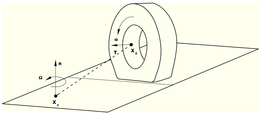
# Procedures description that converts the steady moving contact field problem into a purely spatially dependent simulation. We consider the case shown in Figure 2.7.1-1, where the ground velocity of the body is described in terms of a constant cornering motion. Figure 2.7.1-1 Constant cornering motion. 

text_image

n Ω X₀ ω T X₀

The body is rotating with a constant angular rolling velocity ! around a rigid axle T at ${ \bf { X } } _ { 0 }$ , which in turn rotates with constant angular velocity − around the fixed cornering axis n through point $\mathbf { X } _ { c }$ . Hence, the motion of a particle X at time t consists of a rigid rolling rotation to position $\mathbf { Y } ,$ described by $$ \mathbf {Y} = \mathbf {R} _ {s} \cdot (\mathbf {X} - \mathbf {X} _ {0}) + \mathbf {X} _ {0}, $$ followed by a deformation to point x, and a subsequent cornering rotation (or precession) around n to position y so that $$ \mathbf {y} = \mathbf {R} _ {c} \cdot (\mathbf {x} - \mathbf {X} _ {c}) + \mathbf {X} _ {c}, $$ where $\mathbf { R } _ { c }$ is the cornering rotation given by $\mathbf { R } _ { c } = \exp \left( \hat { \Omega } t \right)$ and $\hat { \Omega }$ is the skew-symmetric matrix associated with the rotation vector $\pmb { \Omega } = \Omega \mathbf { n }$ . Similarly, ${ \bf R } _ { s }$ is the spinning rotation matrix defined as $\mathbf { R } _ { s } = \exp \left( \hat { \pmb { \omega } } t \right)$ and $\hat { \omega }$ is the skew-symmetric matrix associated with the rotation vector ${ \boldsymbol { \omega } } = \omega \mathbf { T }$ . The velocity of the particle then becomes $$ \mathbf {v} = \dot {\mathbf {y}} = \dot {\mathbf {R}} _ {c} \cdot (\mathbf {x} - \mathbf {X} _ {c}) + \mathbf {R} _ {c} \cdot \dot {\mathbf {x}}. $$ To describe the deformation of the body, we define a map $x ( \mathbf { Y } , t )$ , which gives the position of point X at time t as a function of its location Y at time t so that $\mathbf { x } = \pmb { \chi } ( \mathbf { Y } , t )$ : It follows that $$ \dot {\mathbf {x}} = \frac {\partial \pmb {\chi}}{\partial \mathbf {Y}} \cdot \frac {\partial \mathbf {Y}}{\partial t} + \frac {\partial \pmb {\chi}}{\partial t}, $$ where # Procedures $$ \frac {\partial \mathbf {Y}}{\partial t} = \dot {\mathbf {R}} _ {s} \cdot (\mathbf {X} - \mathbf {X} _ {0}) = \omega \mathbf {T} \times (\mathbf {Y} - \mathbf {X} _ {0}). $$ Noting that $\dot { \bf R } _ { s } = \boldsymbol { \hat { \omega } } \cdot { \bf R } _ { s } = \omega \hat { \bf T } \cdot { \bf R } _ { s }$ , and introducing the circumferential direction $\mathbf { S } = \mathbf { T } \times ( \mathbf { Y } - \mathbf { X } _ { 0 } ) / R$ , where $R = | \mathbf { Y } - \mathbf { X } _ { 0 } |$ is the radius of a point on the reference body, the velocity of the reference body can be written as $\partial { \bf Y } / \partial t = \omega R { \bf S }$ , so that $$ \dot {\mathbf {x}} = \omega R \frac {\partial \pmb {\chi}}{\partial \mathbf {Y}} \cdot \mathbf {S} + \frac {\partial \pmb {\chi}}{\partial t} = \omega R \frac {\partial \pmb {\chi}}{\partial S} + \frac {\partial \pmb {\chi}}{\partial t}, $$ where $S = \mathbf { S } \cdot \mathbf { Y }$ is the distance-measuring coordinate along the streamline. Using this result, together with $\begin{array} { r } { \dot { \bf R } _ { c } = \hat { \Omega } \cdot { \bf R } _ { c } = \Omega \hat { \bf n } \cdot { \bf R } _ { c } } \end{array}$ , the velocity of the particle can be written as $$ \mathbf {v} = \Omega \mathbf {n} \times (\mathbf {y} - \mathbf {X} _ {c}) + \omega R \mathbf {R} _ {c} \cdot \frac {\partial \pmb {\chi}}{\partial S} + \mathbf {R} _ {c} \cdot \frac {\partial \pmb {\chi}}{\partial t}. $$ The acceleration is obtained by a second differentiation and some manipulation: $$ \begin{array}{l} \mathbf {a} = \Omega^ {2} (\mathbf {n n} - \mathbf {I}) \cdot (\mathbf {y} - \mathbf {X} _ {c}) + 2 \omega \Omega R \mathbf {n} \times \mathbf {R} _ {c} \cdot \frac {\partial \boldsymbol {\chi}}{\partial S} + 2 \Omega \mathbf {n} \times \mathbf {R} _ {c} \cdot \frac {\partial \boldsymbol {\chi}}{\partial t} \\ + \omega^ {2} R ^ {2} \mathbf {R} _ {c} \cdot \frac {\partial^ {2} \pmb {\chi}}{\partial S ^ {2}} + 2 \omega R \mathbf {R} _ {c} \cdot \frac {\partial^ {2} \pmb {\chi}}{\partial S \partial t} + \mathbf {R} _ {c} \cdot \frac {\partial^ {2} \pmb {\chi}}{\partial t ^ {2}}. \\ \end{array} $$ To obtain expressions for the velocity and acceleration in the reference frame tied to the body, we use the transformations $$ \mathbf {v} _ {r} = \mathbf {R} _ {c} ^ {T} \cdot \mathbf {v} \quad \text {and} \quad \mathbf {a} _ {r} = \mathbf {R} _ {c} ^ {T} \cdot \mathbf {a} $$ so that we obtain $$ \mathbf {v} _ {r} = \Omega \mathbf {n} \times (\mathbf {x} - \mathbf {X} _ {c}) + \omega R \frac {\partial \pmb {\chi}}{\partial S} + \frac {\partial \pmb {\chi}}{\partial t} $$ and $$ \begin{array}{l} \mathbf {a} _ {r} = \Omega^ {2} (\mathbf {n n} - \mathbf {I}) \cdot (\mathbf {x} - \mathbf {X} _ {c}) + 2 \omega \Omega R \mathbf {n} \times \frac {\partial \pmb {\chi}}{\partial S} + 2 \Omega \mathbf {n} \times \frac {\partial \pmb {\chi}}{\partial t} \\ + \omega^ {2} R ^ {2} \frac {\partial^ {2} \pmb {\chi}}{\partial S ^ {2}} + 2 \omega R \frac {\partial^ {2} \pmb {\chi}}{\partial S \partial t} + \frac {\partial^ {2} \pmb {\chi}}{\partial t ^ {2}}. \\ \end{array} $$ For steady-state conditions these expressions reduce to $$ \mathbf {v} _ {r} = \Omega \mathbf {n} \times (\mathbf {x} - \mathbf {X} _ {c}) + \omega R \frac {\partial \pmb {\chi}}{\partial S} $$ and # Procedures $$ \mathbf {a} _ {r} = \Omega^ {2} \left(\mathbf {n n} - \mathbf {I}\right) \cdot \left(\mathbf {x} - \mathbf {X} _ {c}\right) + 2 \omega \Omega R \mathbf {n} \times \frac {\partial \pmb {\chi}}{\partial S} + \omega^ {2} R ^ {2} \frac {\partial^ {2} \pmb {\chi}}{\partial S ^ {2}}. $$ The first term in the last expression can be identified as the acceleration that gives rise to centrifugal forces resulting from rotation about n. Noting that $\omega R \partial \pmb { \chi } / \partial S$ is a measure of velocity, the second term can be identified as the acceleration that gives rise to Coriolis forces. The last term combines the acceleration that gives rise to Coriolis and centrifugal forces resulting from rotation about T. When the deformation is uniform along the circumferential direction, this Coriolis effect vanishes so that the acceleration gives rise to centrifugal forces only. The velocity of the center of the body ${ \bf { X } } _ { 0 }$ (which must lie on the axis T) is $$ \mathbf {v} _ {0} = \boldsymbol {\Omega} \mathbf {n} \times (\mathbf {X} _ {0} - \mathbf {X} _ {c}) $$ since the motions due to rolling and deformation vanish on the axis. 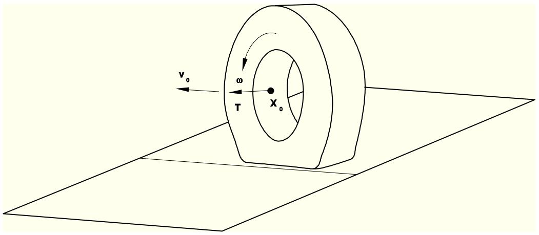To obtain the expression for straight line motion, as shown in Figure 2.7.1-2, we move $\mathbf { X } _ { c }$ far away from the center of the body $\mathbf { x } _ { 0 }$ but keep $\mathbf { v } _ { 0 }$ the same. In that case $\Omega \to 0$ and, hence, in the limit $$ \mathbf {v} = \mathbf {v} _ {0} + \mathbf {v} _ {r} = \mathbf {v} _ {0} + \omega R \frac {\partial \pmb {\chi}}{\partial S}, $$ $$ \mathbf {a} = \mathbf {a} _ {r} = \omega^ {2} R ^ {2} \frac {\partial^ {2} \pmb {\chi}}{\partial S ^ {2}}, $$ which corresponds to straight line rolling. Figure 2.7.1-2 Straight line rolling. 

text_image

v₀ ω T X₀

# Inertia The virtual work contribution from the d'Alembert forces is # Procedures $$ \delta \Pi = - \int_ {V} \rho \mathbf {a} \cdot \delta \mathbf {v} d V. $$ Using the divergence theorem, the virtual work contribution becomes $$ \begin{array}{l} \delta \Pi = - \rho \Omega^ {2} \int_ {V} \left(\mathbf {x} - \mathbf {X} _ {c}\right) \cdot \left(\mathbf {n n} - \mathbf {I}\right) \cdot \delta \mathbf {v} d V - 2 \rho \omega \Omega R \int_ {V} \mathbf {n} \times \frac {\partial \pmb {\chi}}{\partial S} \cdot \delta \mathbf {v} d V \\ + \rho \omega^ {2} R ^ {2} \int_ {V} \frac {\partial \pmb {\chi}}{\partial S} \cdot \frac {\partial \delta \mathbf {v}}{\partial S} d V \\ \end{array} $$ and the rate of virtual work becomes $$ \begin{array}{l} d \delta \Pi = - \rho \Omega^ {2} \int_ {V} d \mathbf {x} \cdot (\mathbf {n n} - \mathbf {I}) \cdot \delta \mathbf {v} d V - 2 \rho \omega \Omega R \int_ {V} \mathbf {n} \times \frac {\partial d \pmb {\chi}}{\partial S} \cdot \delta \mathbf {v} d V \\ + \rho \omega^ {2} R ^ {2} \int_ {V} \frac {\partial d \pmb {\chi}}{\partial S} \cdot \frac {\partial \delta \mathbf {v}}{\partial S} d V. \\ \end{array} $$ For straight line rolling only the last term in each expression needs to be taken into account. # Contact conditions To obtain the contact conditions, we start with the expressions for velocity derived in the previous section. For points on the surface of the deformable body $$ \mathbf {v} _ {D} = \boldsymbol {\Omega} \mathbf {n} \times (\mathbf {x} - \mathbf {X} _ {c}) + \omega R \frac {\partial \pmb {\chi}}{\partial S} + \frac {\partial \pmb {\chi}}{\partial t}, $$ where n is the cornering axis (which must be normal to the rigid surface) and − is the cornering angular velocity around n. Assuming that the velocity of a point on the foundation (or rigid surface) is $\mathbf { v } _ { R }$ , the relative motion becomes $$ \mathbf {v} = \mathbf {v} _ {D} - \mathbf {v} _ {R} = \Omega \mathbf {n} \times \mathbf {r} + \omega R \frac {\partial \pmb {\chi}}{\partial S} + \frac {\partial \pmb {\chi}}{\partial t} - \mathbf {v} _ {R}, $$ where $\mathbf { r } = \mathbf { x } - \mathbf { X } _ { c }$ . This equation can be split into normal and tangential components. The rate of penetration is $$ \dot {h} = - \mathbf {n} \cdot \mathbf {v} = \mathbf {n} \cdot \mathbf {v} _ {R} - \omega R \mathbf {n} \cdot \frac {\partial \pmb {\chi}}{\partial S} - \mathbf {n} \cdot \frac {\partial \pmb {\chi}}{\partial t}. $$ For any point in contact n ¢ $\partial \pmb { \chi } / \partial S = 0 ;$ hence, $$ \dot {h} = \mathbf {n} \cdot \mathbf {v} _ {R} - \mathbf {n} \cdot \frac {\partial \pmb {\chi}}{\partial t}, $$ which in incremental form reduces to the standard contact condition # Procedures $$ \Delta h = \mathbf {n} \cdot (\Delta \mathbf {x} _ {R} - \Delta \mathbf {x} _ {D}). $$ For steady-state conditions n ¢ $\Delta { \bf x } _ { R } = 0$ and $\Delta { \bf x } _ { D } = 0$ . Similarly, the rate of slip is $$ \dot {\gamma} _ {\alpha} = \mathbf {t} _ {\alpha} \cdot \mathbf {v} = \Omega \mathbf {t} _ {\alpha} \cdot (\mathbf {n} \times \mathbf {r}) + \omega R \mathbf {t} _ {\alpha} \cdot \frac {\partial \pmb {\chi}}{\partial S} + \mathbf {t} _ {\alpha} \cdot \frac {\partial \pmb {\chi}}{\partial t} - \mathbf {t} _ {\alpha} \cdot \mathbf {v} _ {R}, $$ where ${ \bf t } _ { \alpha } \left( \alpha = 1 , 2 \right)$ are two orthogonal unit vectors tangent to the contact surface so that $\mathbf { n } = \mathbf { t } _ { 1 } \times \mathbf { t } _ { 2 }$ . For steady-state conditions $\partial \pmb { \chi } / \partial t = 0$ , so $$ \dot {\gamma} _ {\alpha} = \mathbf {t} _ {\alpha} \cdot \mathbf {v} = \Omega \mathbf {t} _ {\alpha} \cdot (\mathbf {n} \times \mathbf {r}) + \omega R \mathbf {t} _ {\alpha} \cdot \frac {\partial \boldsymbol {\chi}}{\partial S} - \mathbf {t} _ {\alpha} \cdot \mathbf {v} _ {R}. $$ Variations in $\dot { \gamma } _ { \alpha }$ yield $$ \delta \dot {\gamma} _ {\alpha} = \Omega \mathbf {t} _ {\alpha} \cdot (\mathbf {n} \times \delta \mathbf {r}) + \omega R \mathbf {t} _ {\alpha} \cdot \frac {\partial \delta \pmb {\chi}}{\partial S} - \mathbf {t} _ {\alpha} \cdot \delta \mathbf {v} _ {R}. $$ For straight line rolling we can replace − n £ r by $\mathbf { v } _ { 0 }$ so that we obtain $$ \dot {\gamma} _ {\alpha} = \mathbf {t} _ {\alpha} \cdot \mathbf {v} _ {0} + \omega R \mathbf {t} _ {\alpha} \cdot \frac {\partial \pmb {\chi}}{\partial S} - \mathbf {t} _ {\alpha} \cdot \mathbf {v} _ {R} $$ and $$ \delta \dot {\gamma} _ {\alpha} = \omega R \mathbf {t} _ {\alpha} \cdot \frac {\partial \delta \boldsymbol {\chi}}{\partial S} - \mathbf {t} _ {\alpha} \cdot \delta \mathbf {v} _ {R}. $$ To complete the formulation, a relationship between frictional stress and slip velocity must be developed. A Coulomb friction law is provided for steady-state rolling. The law assumes that slip occurs if the frictional stress, $$ \tau_ {e q} = \sqrt {\tau_ {1} ^ {2} + \tau_ {2} ^ {2}}, $$ is equal to the critical stress, $\tau _ { c r i t } = \mu p _ { ; }$ , where $\tau _ { 1 }$ and $\tau _ { 2 }$ are shear stresses along $\mathbf { t } _ { \alpha } , \mu$ is the friction coefficient, and p is the contact pressure. On the other hand, when $\tau _ { e q } < \tau _ { c r i t }$ , no relative motion occurs. The condition of no relative motion is approximated in ABAQUS by stiff viscous behavior $$ \tau_ {\alpha} = \kappa_ {s} \dot {\gamma} _ {\alpha} ^ {v}, $$ where $\dot { \gamma } _ { \alpha }$ is the tangential slip velocity and $\kappa _ { s }$ is the "stick viscosity," which follows from the relation $$ \kappa_ {s} = \frac {\tau_ {c r i t}}{\dot {\gamma} _ {c r i t}}. $$ The allowable viscous slip velocity is defined as a fraction of the circumferential velocity $$ \dot {\gamma} _ {c r i t} = 2 F _ {f} \omega R, $$ where $F _ { f }$ is a user-defined slip tolerance. These expressions contribute to the standard virtual work contribution for slip, $$ \delta \Pi = \int_ {A} \tau_ {\alpha} \delta \gamma_ {\alpha} d A, $$ and rate of virtual work for slip, $$ d \delta \Pi = \int_ {A} \left(\mathrm{d} \tau_ {\alpha} \delta \gamma_ {\alpha} + \tau_ {\alpha} \mathrm{d} \delta \gamma_ {\alpha}\right) d A. $$ # 2.8 Analysis of porous media # 2.8.1 Effective stress principle for porous media A porous medium is modeled in ABAQUS/Standard by the conventional approach that considers the medium as a multiphase material and adopts an effective stress principle to describe its behavior. The porous medium modeling provided considers the presence of two fluids in the medium. One is the "wetting liquid," which is assumed to be relatively (but not entirely) incompressible. Often the other is a gas, which is relatively compressible. An example of such a system is soil containing ground water. When the medium is partially saturated, both fluids exist at a point: when it is fully saturated, the voids are completely filled with the wetting liquid. The elementary volume, $d V$ , is made up of a volume of grains of solid material, $d V _ { g } ;$ ; a volume of voids, $d V _ { v }$ ; and a volume of wetting liquid, $d V _ { w } \leq d V _ { v }$ , that is free to move through the medium if driven. In some systems (for example, systems containing particles that absorb the wetting liquid and swell in the process) there may also be a significant volume of trapped wetting liquid, $d V _ { t }$ . The total stress acting at a point, $\sigma ,$ is assumed to be made up of an average pressure stress in the wetting liquid, $u _ { w }$ , called the "wetting liquid pressure," an average pressure stress in the other fluid, $u _ { a }$ , and an "effective stress, $" \overline { { \sigma } } ^ { * }$ , defined by Equation 2.8.1-1 $$ \overline {{{\boldsymbol {\sigma}}}} ^ {*} = \boldsymbol {\sigma} + \left(\chi u _ {w} + (1 - \chi) u _ {a}\right) \mathbf {I}. $$ Stress components are stored so that tensile stress is positive, but $u _ { w }$ and $u _ { a }$ are pressure stress values. This explains the sign in this equation. $\chi$ is a factor that depends on saturation and on the surface tension of the liquid/solid system (Wu, 1976). Â is 1.0 when the medium is fully saturated and between 0.0 and 1.0 in unsaturated systems when its value depends on the degree of saturation of the medium. There is very sparse experimental evidence of its dependence on saturation; and because of this lack of # Procedures data, we simply assume that $\chi$ is equal to the saturation of the medium (we define saturation later in this section). We simplify the model by assuming that the pressure applied to the nonwetting fluid is constant throughout the domain being modeled, does not vary with time, and is small enough that its value can be neglected. This requires that the nonwetting fluid can diffuse through the medium sufficiently freely so that its pressure, $u _ { a ; }$ , never exceeds the pressure applied to this fluid at the boundaries of the medium, which remains constant throughout the process being modeled. The most common example where this simplification applies is a porous medium that is quite permeable to gas flow, in which the nonwetting fluid is air, exposed to atmospheric pressure. The dimensions of the region modeled must not be so large that the gravitational gradient of atmospheric pressure causes a significant change in the air pressure, and there can be no external event that provides a transient change in the air pressure. This assumption allows $u _ { a }$ to be removed from the equation, provided that the corresponding loading term (for example, atmospheric pressure on the boundary of the medium) is also omitted from the equilibrium equations and that $u _ { a }$ is small enough that its effect on the deformation of the medium is not important (or that deformation is measured from the state $\pmb { \sigma } = - u _ { a } \mathbf { I } )$ . This simplification reduces the effective stress principle to Equation 2.8.1-2 $$ \overline {{\pmb {\sigma}}} ^ {*} = \pmb {\sigma} + \chi u _ {w} \mathbf {I}. $$ In the case where trapped fluid is present in the system, we assume that the effective stress is made up of two components weighted according to the relative volume of trapped fluid and porous material: Equation 2.8.1-3 $$ \overline {{\pmb {\sigma}}} ^ {*} = (1 - n _ {t}) \overline {{\pmb {\sigma}}} - n _ {t} \overline {{p}} _ {t} \mathbf {I}, $$ where $\overline { { \pmb { \sigma } } }$ is the effective stress in the porous material skeleton, $\overline { { p } } _ { t }$ is the average pressure stress in the trapped liquid, and $n _ { t }$ is the ratio of trapped fluid volume to total volume, as defined later in this section. We assume that the constitutive response of the porous medium consists of simple bulk elasticity relationships for the liquid and for the soil grains, together with a constitutive theory for the soil skeleton whereby $\overline { { \pmb { \sigma } } }$ is defined as a function of the strain history and temperature of the soil: $\overline { { \pmb { \sigma } } } = \overline { { \pmb { \sigma } } }$ (strain history, temperature, state variables ): Constitutive models that are appropriate for voided materials, such as soils, are described in Chapter 4, "Mechanical Constitutive Theories." The remaining parts of \`\`Analysis of porous media,'' Section 2.8, discuss the equilibrium equation for porous media (\`\`Discretized equilibrium statement for a porous medium,'' Section 2.8.2), fundamental constitutive assumptions that incorporate the effective stress principle as outlined above (\`\`Constitutive behavior in a porous medium, '' Section 2.8.3), and the continuity equation that governs the flow of the wetting liquid (\`\`Continuity statement for the wetting liquid phase in a porous # Procedures medium,'' Section 2.8.4). Newton's method is generally used to solve the governing equations for the implicit time integration procedure. Analysis of small, linearized, perturbations about a deformed state is also sometimes required (for vibration studies, for example). For these reasons the development includes a definition of the form of the Jacobian matrix for the two-phase model. As preliminaries, porosity, void ratio, and saturation are defined. The porosity of the medium, n, is the ratio of the volume of voids to the total volume: $$ n \stackrel {\mathrm{def}} {=} \frac {d V _ {v}}{d V} = 1 - \frac {d V _ {g}}{d V} - \frac {d V _ {t}}{d V}. $$ Using the superscript 0 to indicate values in some convenient reference configuration allows the porosity in the current configuration to be expressed as $$ \begin{array}{l} n = 1 - \frac {d V _ {g}}{d V _ {g} ^ {0}} \frac {d V ^ {0}}{d V} \frac {d V _ {g} ^ {0}}{d V ^ {0}} - \frac {d V _ {t}}{d V} \\ = 1 - J _ {g} J ^ {- 1} (1 - n ^ {0} - n _ {t} ^ {0}) - n _ {t}, \\ \end{array} $$ so that Equation 2.8.1-4 $$ \frac {1 - n - n _ {t}}{1 - n ^ {0} - n _ {t} ^ {0}} = \frac {J _ {g}}{J}, $$ where $$ J \stackrel {\mathrm{def}} {=} \left| \frac {d V}{d V ^ {0}} \right| $$ is the ratio of the medium's volume in the current configuration to its volume in the reference configuration, $$ J _ {g} \stackrel {\mathrm{def}} {=} \left| \frac {d V _ {g}}{d V _ {g} ^ {0}} \right| $$ is the ratio of the current to reference volume for the grains, and $$ n _ {t} \stackrel {\mathrm{def}} {=} \frac {d V _ {t}}{d V} $$ is the volume of trapped wetting liquid per unit of current volume. ABAQUS generally uses void ratio, $e \ { \stackrel { \mathrm { d e f } } { = } } \ d V _ { v } / ( d V _ { g } + d V _ { t } )$ , instead of porosity. Conversion relationships are readily derived as Equation 2.8.1-5 # Procedures $$ e = \frac {n}{1 - n}, \quad n = \frac {e}{1 + e}, \quad 1 - n = \frac {1}{1 + e}. $$ Saturation, s, is the ratio of free (untrapped) wetting liquid volume to void volume: $$ s \stackrel {\mathrm{def}} {=} \frac {d V _ {w}}{d V _ {v}}. $$ The volume ratio of free wetting liquid at a point is $$ n _ {w} \stackrel {\mathrm{def}} {=} \frac {d V _ {w}}{d V} = s n. $$ The total volume of wetting liquid (free liquid plus trapped liquid) per unit of current volume is $$ n _ {f} = s n + n _ {t}. $$ # 2.8.2 Discretized equilibrium statement for a porous medium Equilibrium is expressed by writing the principle of virtual work for the volume under consideration in its current configuration at time t: $$ \int_ {V} \pmb {\sigma}: \delta \pmb {\varepsilon} d V = \int_ {S} \mathbf {t} \cdot \delta \mathbf {v} d S + \int_ {V} \hat {\mathbf {f}} \cdot \delta \mathbf {v} d V, $$ where $\delta \mathbf { v }$ is a virtual velocity field, $\delta \pmb { \varepsilon } \overset { \mathrm { d e f } } { = } \mathrm { s y m } ( \partial \delta \mathbf { v } / \partial \mathbf { x } )$ is the virtual rate of deformation, $\pmb { \sigma }$ is the true (Cauchy) stress, t are surface tractions per unit area, and $\hat { \mathbf { f } }$ are body forces per unit volume. For our system $\hat { \mathbf { f } }$ will often include the weight of the wetting liquid, $$ \mathbf {f} _ {w} = (s n + n _ {t}) \rho_ {w} \mathbf {g}, $$ where $\rho _ { w }$ is the density of the wetting liquid and g is the gravitational acceleration, which we assume to be constant and in a constant direction (so that, for example, the formulation cannot be applied directly to a centrifuge experiment unless the model in the machine is small enough that g can be treated as constant). For simplicity we consider this loading explicitly so that any other gravitational term in ^f is associated only with the weight of the dry porous medium. Thus, we write the virtual work equation as Equation 2.8.2-1 $$ \int_ {V} \pmb {\sigma}: \delta \pmb {\varepsilon} d V = \int_ {S} \mathbf {t} \cdot \delta \mathbf {v} d S + \int_ {V} \mathbf {f} \cdot \delta \mathbf {v} d V + \int_ {V} (s n + n _ {t}) \rho_ {w} \mathbf {g} \cdot \delta \mathbf {v} d V, $$ where f are all body forces except the weight of the wetting liquid. In a finite element model equilibrium is approximated as a finite set of equations by introducing # Procedures interpolation functions. The notation used to indicate such discretization are those quantities with uppercase superscripts (for example, $v ^ { N } )$ , which represent nodal variables, with the summation convention adopted for the superscripts. The interpolation is assumed to be based on material coordinates in the material skeleton (a "Lagrangian" formulation). For simplicity, in this section we consider only the case where the problem has no internal constraints--such as incompressibility--and the discretization is made entirely by approximating equilibrium: this results in the displacement (or stiffness) method. Mixed formulation ("hybrid") elements are available for porous medium analysis with ABAQUS/Standard, but consideration of such formulations does not require any important extension of the development at this stage. The virtual velocity field is interpolated by $$ \delta \mathbf {v} = \mathbf {N} ^ {N} \delta v ^ {N}, $$ where $\mathbf { N } ^ { N } ( S _ { i } )$ are interpolation functions defined with respect to material coordinates, $S _ { i }$ The virtual rate of deformation is interpolated as $$ \delta \boldsymbol {\varepsilon} = \boldsymbol {\beta} ^ {N} \delta v ^ {N}, $$ where, in the simplest case, $$ \pmb {\beta} ^ {N} = \mathrm{sym} \left(\frac {\partial \delta \mathbf {N} ^ {N}}{\partial \mathbf {x}}\right), $$ although more general forms are used in some of the elements in ABAQUS. The virtual work equation is thus discretized as $$ \delta v ^ {N} \int_ {V} \pmb {\beta} ^ {N}: \pmb {\sigma} d V = \delta v ^ {N} \left[ \int_ {S} \mathbf {N} ^ {N} \cdot \mathbf {t} d S + \int_ {V} \mathbf {N} ^ {N} \cdot \mathbf {f} d V + \int_ {V} (s n + n _ {t}) \rho_ {w} \mathbf {N} ^ {N} \cdot \mathbf {g} d V \right], $$ where the $\delta v ^ { N }$ are assumed to be independent. The term conjugate to $\delta v ^ { N }$ on the left-hand side of this equation is referred to subsequently as the internal force array, $I ^ { N }$ : $$ I ^ {N} \stackrel {\text { def }} {=} \int_ {V} \boldsymbol {\beta} ^ {N}: \boldsymbol {\sigma} d V. $$ Likewise, the external force array, $P ^ { N }$ , is taken from the right-hand side: $$ P ^ {N} \stackrel {\mathrm{def}} {=} \int_ {S} \mathbf {N} ^ {N} \cdot \mathbf {t} d S + \int_ {V} \mathbf {N} ^ {N} \cdot \mathbf {f} d V + \int_ {V} (s n + n _ {t}) \rho_ {w} \mathbf {N} ^ {N} \cdot \mathbf {g} d V $$ $( P ^ { N }$ includes any d'Alembert forces).