compared to the time history of interest in such cases that the explicit method is very economic. Cormeau (1975) has developed formulae for the stability limit for most common cases of stress induced creep, and these results are used to monitor stability. For this explicit approach the integration is trivial. Combining the integrated flow rule $$ \Delta \pmb {\varepsilon} ^ {p l} = \Delta t \frac {\partial G _ {c r}}{\partial \pmb {\sigma}} | _ {t} $$ with the integrated strain rate decomposition and the (linear) elasticity gives Equation 4.3.4-1 $$ \pmb {\sigma} | _ {t + \Delta t} = \mathbf {D} ^ {e l}: \left(\varepsilon_ {t + \Delta t} - \varepsilon^ {p l} | _ {t} - \Delta t \left. \frac {\partial G _ {c r}}{\partial \pmb {\sigma}} \right| _ {t}\right). $$ All of the terms on the right-hand side of this set of equations are known when the constitutive integration is done, so these equations define $\pmb { \sigma } _ { t + \Delta t }$ explicitly. There also exist many problems involving rate-dependent plastic response in which the characteristic relaxation times for the material under the stress states to which it is subjected are very short compared to the time period of interest in the analysis, so the conditional stability of the explicit operator will only allow very short time increments. For such cases it can be more economical to use the backward Euler method because of its unconditional stability. ABAQUS always uses the implicit method for high strain rate applications to avoid time increment restrictions being introduced by considerations of stability in the integration of the constitutive model. ABAQUS will also use the implicit method in all geometrically nonlinear problems and in problems for which rate-independent plasticity is active simultaneously. The backward Euler method is implicit; and because the plastic strain rate is usually a strong function of stress, some care must be taken to develop an effective algorithm to solve the nonlinear algebraic equations that result from the use of this operator. The problem has been posed formally in \`\`Integration of plasticity models,'' Section 4.2.2. The main difficulty is to obtain a reasonable starting guess for $\Delta \varepsilon ^ { p l }$ . For this we proceed as follows. For simplicity, we consider rate-dependent behavior only and the particular form of flow rule defined by $$ \dot {\pmb {\varepsilon}} ^ {p l} = \dot {\overline {{\varepsilon}}} ^ {s w} \frac {1}{3} \mathbf {I} + \dot {\overline {{\varepsilon}}} ^ {c r} \mathbf {n}, $$ where $\dot { \overline { { \mathcal { E } } } } ^ { s w }$ is the "equivalent swelling strain rate," $\dot { \bar { \varepsilon } } ^ { c r }$ is the "equivalent creep strain rate," and n is the gradient of the deviatoric stress potential, $$ \mathbf {n} = \frac {\partial \tilde {q}}{\partial \pmb {\sigma}}, $$ where $\tilde { q }$ is the Mises or Hill stress potential (defined in \`\`Stress potentials for anisotropic metal # Mechanical Constitutive Theories plasticity,'' Section 4.3.3). The "equivalent strain rates" are part of the stress potential for the plastic response and, therefore, are assumed to have evolution laws of the form $$ \dot {\overline {{\varepsilon}}} ^ {s w} = h ^ {s} (p, \tilde {q}, \overline {{\varepsilon}} ^ {s w}, \overline {{\varepsilon}} ^ {c r}, \theta , \dots) $$ and $$ \dot {\overline {{\varepsilon}}} ^ {c r} = h ^ {c} (p, \tilde {q}, \overline {{\varepsilon}} ^ {s w}, \overline {{\varepsilon}} ^ {c r}, \theta , \dots). $$ Backward Euler integration of the flow equation gives $$ \Delta \pmb {\varepsilon} ^ {p l} = \Delta \overline {{\varepsilon}} ^ {s w} \frac {1}{3} \mathbf {I} + \Delta \overline {{\varepsilon}} ^ {c r} \mathbf {n}, $$ where n is understood to be evaluated at time $t + \Delta t .$ , and Equation 4.3.4-2 $$ \Delta \overline {{\varepsilon}} ^ {s w} = \Delta t h ^ {s} (p, \tilde {q}, \overline {{\varepsilon}} ^ {s w}, \overline {{\varepsilon}} ^ {c r}, \theta , \dots) $$ and $$ \Delta \overline {{\varepsilon}} ^ {c r} = \Delta t h ^ {c} (p, \tilde {q}, \overline {{\varepsilon}} ^ {s w}, \overline {{\varepsilon}} ^ {c r}, \theta , \dots). $$ Equation 4.3.4-3 $\Delta \overline { { \varepsilon } } ^ { c r }$ and $\Delta \overline { { \varepsilon } } ^ { s w }$ are usually defined in user subroutine CREEP. The solution to the algebraic problem is obtained by first finding reasonable initial guesses for $\Delta \overline { { \varepsilon } } ^ { c r }$ and $\Delta \varepsilon ^ { s w }$ and then solving the full problem. The Mises and Hill equivalent stress definitions ( q\~) both have the property that $$ \mathbf {n}: \boldsymbol {\sigma} = \tilde {q}. $$ We also have the simple relationship $$ \mathbf {I}: \boldsymbol {\sigma} = - 3 p. $$ The initial estimates for $\Delta \varepsilon ^ { c r }$ and $\Delta \varepsilon ^ { s w }$ are obtained by projecting the problem onto $\mathbf { n } ^ { e l }$ and I, where $\mathbf { n } ^ { e l }$ is $\partial \tilde { q } / \partial \pmb { \sigma }$ defined at ${ \pmb \sigma } ^ { e l }$ , the stress state that would arise at the end of the increment if there were no inelastic deformation during the increment. The projections are Equation 4.3.4-4 $$ \tilde {q} = \tilde {q} ^ {e l} - G \Delta \overline {{\varepsilon}} ^ {c r} - B \Delta \overline {{\varepsilon}} ^ {s w}, $$ and Equation 4.3.4-5 $$ p = p ^ {e l} - B \Delta \overline {{\varepsilon}} ^ {c r} - K \Delta \overline {{\varepsilon}} ^ {s w}, $$ where $$ \tilde {q} ^ {e l} = \mathbf {n}: \pmb {\sigma} ^ {e l}, $$ $$ p ^ {e l} = - \frac {1}{3} \mathbf {I}: \pmb {\sigma} ^ {e l}, $$ $$ G = \mathbf {n}: \mathbf {D} ^ {e l}: \mathbf {n}, $$ $$ K = \frac {1}{9} \mathbf {I}: \mathbf {D} ^ {e l}: \mathbf {I}, $$ and $$ B = \frac {1}{3} \mathbf {n} ^ {e l}: \mathbf {D} ^ {e l}: \mathbf {I}. $$ Equation 4.3.4-2 to Equation 4.3.4-5 are a set of nonlinear equations that can be solved for $\Delta \varepsilon ^ { c r }$ and $\Delta \varepsilon ^ { s w }$ . We solve these equations by Newton's method and then use this solution as the starting estimate for solving the complete problem. When the Mises stress potential is used and the problem is not plane stress, this starting estimate is the solution to the complete problem because the Mises stress potential is a circle in the deviatoric plane. # 4.3.5 Models for metals subjected to cyclic loading The kinematic hardening models in ABAQUS are intended to simulate the behavior of metals that are subjected to cyclic loading. These models are typically applied to studies of low-cycle fatigue and ratchetting. The basic concept of these models is that the yield surface shifts in stress space so that straining in one direction reduces the yield stress in the opposite direction, thus simulating the Bauschinger effect and anisotropy induced by work hardening. Two kinematic hardening models are available in ABAQUS. The simplest model provides linear kinematic hardening and is, thus, mainly used for low-cycle fatigue evaluations. This model yields physically reasonable results if the uniaxial behavior is linearized in the plastic range (a constant work-hardening slope). This is usually best accomplished by guessing the strain levels that will be attained in the problem and linearizing the actual material behavior accordingly. It is important to recognize this restriction on the theory's ability to provide reasonable results and to provide material data accordingly. This model is available with the Mises or Hill yield surface. The combined isotropic/kinematic hardening model is an extension of the linear model. It provides a more accurate approximation to the stress-strain relation than the linear model. It also models other phenomena--such as ratchetting, relaxation of the mean stress, and cyclic hardening--that are typical of materials subjected to cyclic loading. This model is available only with the Mises yield surface. This section first describes those aspects of the formulation that are common to both models; the specific formulation of each model is presented subsequently. # Strain rate decomposition The total strain rate "\_ is written in terms of the elastic and plastic strain rates as Equation 4.3.5-1 $$ \dot {\varepsilon} = \dot {\varepsilon} ^ {e l} + \dot {\varepsilon} ^ {p l}. $$ # Elastic behavior The elastic behavior can be modeled only as linear elastic Equation 4.3.5-2 $$ \pmb {\sigma} = \mathbf {D} ^ {e l}: \pmb {\varepsilon}, $$ where $\mathbf { D } ^ { e l }$ represents the fourth-order elasticity tensor and ¾ and " are the second-order stress and strain tensors, respectively. # Plastic behavior The models are pressure-independent plasticity models. For both models the yield surface is defined by the function Equation 4.3.5-3 $$ f (\pmb {\sigma} - \pmb {\alpha}) = \sigma^ {0}, $$ where $f ( { \pmb \sigma } - { \pmb \alpha } )$ is the equivalent Mises stress or Hill's potential with respect to the backstress or "kinematic shift" ®, and $\sigma ^ { 0 }$ is the size of the yield surface. For instance, the equivalent Mises stress is defined as $$ f (\pmb {\sigma} - \pmb {\alpha}) = \sqrt {\frac {3}{2} \left(\mathbf {S} - \pmb {\alpha} ^ {d e v}\right) : \left(\mathbf {S} - \pmb {\alpha} ^ {d e v}\right)}, $$ Equation 4.3.5-4 where $\pmb { \alpha } ^ { d e v }$ is the deviatoric part of the backstress and S is the deviatoric stress tensor. These models assume associated plastic flow: Equation 4.3.5-5 $$ \dot {\pmb {\varepsilon}} ^ {p l} = \frac {\partial f (\pmb {\sigma} - \pmb {\alpha})}{\partial \pmb {\sigma}} \dot {\bar {\varepsilon}} ^ {p l}, $$ where $\dot { \varepsilon } ^ { p l }$ represents the rate of plastic flow and $\dot { \bar { \varepsilon } } ^ { p l }$ is the equivalent plastic strain rate, "¹\_ pl $\dot { \bar { \varepsilon } } ^ { p l } = \sqrt { \frac { 2 } { 3 } \dot { \bar { \varepsilon } } ^ { p l } : \dot { \varepsilon } ^ { p l } }$ : # Linear kinematic hardening model This model is the simpler of the two kinematic hardening models available in ABAQUS. The size of the yield surface, $\sigma ^ { 0 } ( \theta )$ , can be a function of temperature only for this model. The evolution of ® is defined by Ziegler's hardening rule, generalized to the nonisothermal case as Equation 4.3.5-6 $$ \dot {\pmb {\alpha}} = C \dot {\bar {\varepsilon}} ^ {p l} \frac {1}{\sigma^ {0}} (\pmb {\sigma} - \pmb {\alpha}) + \frac {1}{C} \pmb {\alpha} \dot {C}, $$ where $C ( \theta )$ is the hardening parameter $( C ( \theta )$ is the work-hardening slope of the isothermal uniaxial stress-strain response, $d \sigma / d \bar { \varepsilon } ^ { p l }$ , taken at different temperatures) and $\dot { C }$ is the rate of change of C with respect to temperature. This form of evolution law for ® defines the rate of ® due to plastic straining to be in the direction of the current radius vector from the center of the yield surface, ${ \pmb \sigma } - { \pmb \alpha } ,$ , and the rate due to temperature changes to be toward the origin of stress space. Rice (1975) writes this concept quite generally as Equation 4.3.5-7 $$ \dot {\boldsymbol {\alpha}} = \dot {\mu} (\boldsymbol {\sigma} - \boldsymbol {\alpha}) + h \boldsymbol {\alpha} \dot {\theta}. $$ The particular identification of $\dot { \mu } = C \dot { \bar { \varepsilon } } ^ { p l } / \sigma ^ { 0 }$ and $h = ( d C / d \theta ) / C$ in Equation 4.3.5-6 above is assumed, so the material behavior is defined by the isothermal, uniaxial work hardening data, $C ( \theta )$ only. # Nonlinear isotropic/kinematic hardening model This model is based on the work of Lemaitre and Chaboche (1990). The size of the yield surface, $\sigma ^ { 0 } ( \bar { \varepsilon } ^ { p l } , \theta , f _ { i } )$ , is defined as a function of equivalent plastic strain, $\bar { \varepsilon } ^ { p l } ;$ temperature, $\theta ;$ and field variables, $f _ { i }$ . This dependency can be provided directly, can be coded in user subroutine UHARD, or can be modeled with a simple exponential law for materials that either cyclically harden or soften as Equation 4.3.5-8 $$ \sigma^ {0} = \sigma | _ {0} + Q _ {\infty} (1 - e ^ {- b \bar {\varepsilon} ^ {p l}}), $$ where $\sigma | _ { 0 } ( \theta , f _ { i } )$ is the yield surface size at zero plastic strain, and $Q _ { \infty } ( \theta , f _ { i } )$ and $b ( \theta , f _ { i } )$ are additional material parameters that must be calibrated from cyclic test data. The evolution of the kinematic component of the model is defined as Equation 4.3.5-9 $$ \dot {\pmb {\alpha}} = C \dot {\bar {\varepsilon}} ^ {p l} \frac {1}{\sigma^ {0}} (\pmb {\sigma} - \pmb {\alpha}) - \gamma \pmb {\alpha} \dot {\bar {\varepsilon}} ^ {p l} + \frac {1}{C} \pmb {\alpha} \dot {C}, $$ where $C$ and $\gamma$ are material parameters, with $\dot { C }$ representing the rate of change of $C$ with respect to temperature and field variables. The rate of change of $\gamma$ with respect to temperature and field variables is not accounted for in the model. This equation is the basic Ziegler law, generalized to account for temperature and field variable dependency of C and to which a "recall" term, $\gamma \pmb { \alpha } \dot { \bar { \varepsilon } } ^ { p l }$ , has been added. The recall term introduces the nonlinearity in the evolution law. The evolution of the backstress and the isotropic hardening are illustrated in Figure 4.3.5-1 for unidirectional loading and in Figure 4.3.5-2 for multiaxial loading. Figure 4.3.5-1 One-dimensional representation of the nonlinear model. 

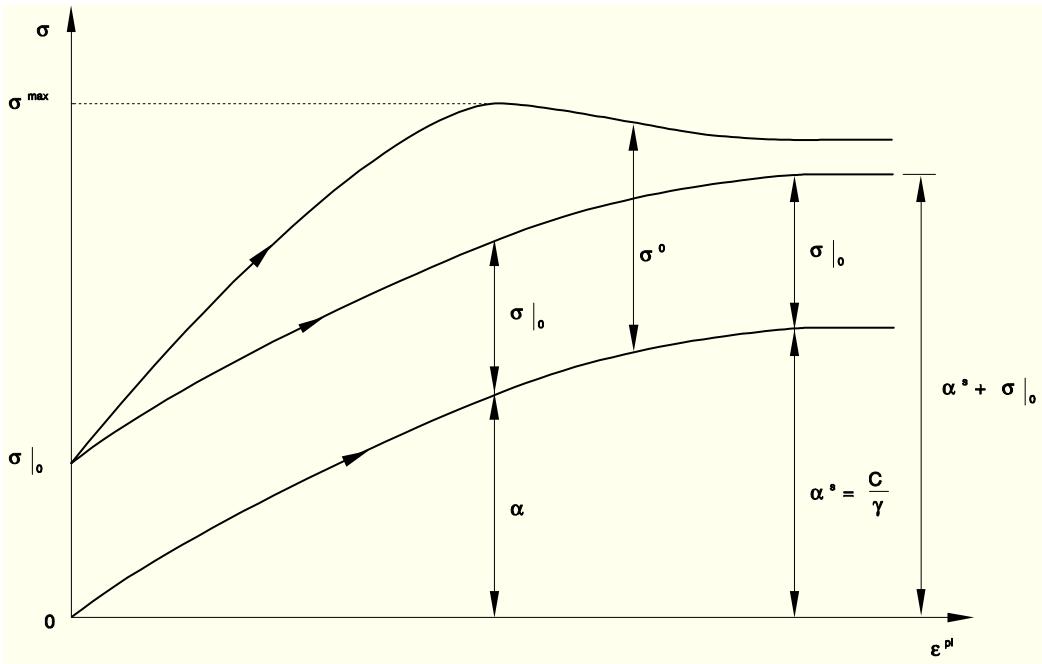
line

| ε^pl | σ_max | σ_0 | σ_10 | σ_20 | |------|-------|-----|------|------| | 0 | 0 | 0 | 0 | 0 | | α | σ_max | σ_0 | σ_10 | σ_20 | | α² = C/γ | σ_max | σ_0 | σ_10 | σ_20 |

Figure 4.3.5-2 Three-dimensional representation of the nonlinear model. 

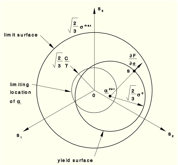
text_image

lim it surface √2/3 σmax √2/3 C/γ ∂F/∂σ S 0 αdev √2/3 σ0 S1 yield surface S2 S3

The center of the yield surface is contained within a cylinder of radius ${ \sqrt { 2 / 3 } } C / \gamma$ , which follows directly from Equation 4.3.5-9. Therefore, the yield surface is contained within the limiting surface of radius ${ \sqrt { 2 / 3 } } \sigma ^ { m a x }$ , as shown in the figures. This model can be degenerated into the linear kinematic model described above by setting $\sigma ^ { 0 } = \sigma | _ { 0 }$ and $\gamma = 0$ . The physical behavior that can be captured by this model, as well as its limitations, is described in detail in the ABAQUS/Standard User's Manual. # 4.3.6 Porous metal plasticity The porous metal plasticity model is intended for use with mildly voided metals. Even though the material that contains the voids (also known as the matrix material) is assumed to be plastically incompressible, the plastic behavior of the bulk material is pressure-dependent due to the presence of voids. The model is described in the following paragraphs, followed by a brief description of the material point calculations. # Yield condition For a metal containing a dilute concentration of voids, based on a rigid-plastic upper bound solution for spherically symmetric deformations of a single spherical void, Gurson (1977) proposed a yield condition of the form $$ \phi = \left(\frac {q}{\sigma_ {y}}\right) ^ {2} + 2 q _ {1} f \cosh \left(- \frac {3}{2} \frac {q _ {2} p}{\sigma_ {y}}\right) - (1 + q _ {3} f ^ {2}) = 0, $$ where $$ \mathbf {S} = p \mathbf {I} + \pmb {\sigma} $$ is the deviatoric part of the macroscopic Cauchy stress tensor $\sigma ;$ $$ q = \sqrt {\frac {3}{2} \mathbf {S} : \mathbf {S}} $$ is the Mises stress; $$ p = - \frac {1}{3} \pmb {\sigma}: \mathbf {I} $$ is the hydrostatic pressure; f is the volume fraction of the voids in the material; and $\sigma _ { y } \big ( \bar { \varepsilon } _ { m } ^ { p l } \big )$ is the yield stress of the fully dense matrix material as a function of $\bar { \varepsilon } _ { m } ^ { p l }$ , the equivalent plastic strain in the matrix. Tvergaard (1981) introduced the constants $q _ { 1 } , q _ { 2 } ,$ , and $q _ { 3 } = q _ { 1 } ^ { 2 }$ (as coefficients of the void volume fraction and pressure terms) to make the predictions of the Gurson model agree with numerical studies of "ordered" voided materials in plane strain tensile fields; one can recover the original Gurson model by setting $q _ { 1 } = q _ { 2 } = q _ { 3 } = 1$ . It should be noted that f = 0 implies that the material is fully dense, and the Gurson yield condition reduces to that of von Mises; f = 1 implies that the material is fully voided and has no stress carrying capacity. This is illustrated in Figure 4.3.6-1, where the yield surfaces for different levels of porosity are shown in the $p – q$ plane. Figure 4.3.6-2 compares the behavior of a porous metal (which has an initial void volume fraction of $f _ { 0 } )$ in tension and compression against the perfectly plastic matrix material; the initial yield stress of the porous metal is $\sigma _ { y _ { 0 } }$ . In compression the porous material "hardens" due to closing of the voids, and in tension it "softens" due to growth and nucleation of the voids. Figure 4.3.6-1 Schematic of the yield surface in the p-q plane.  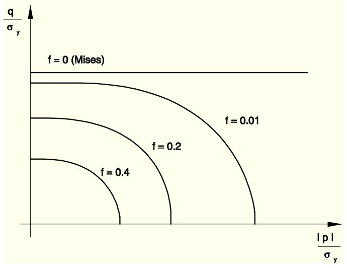Figure 4.3.6-2 Schematic of uniaxial behavior of a porous metal. 

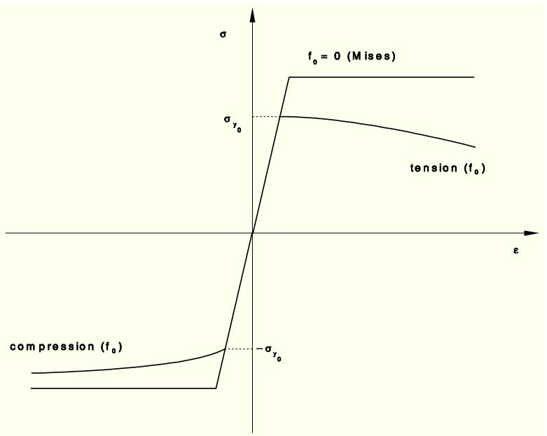
line

| ε | σ (f₀ = 0) | σ (tension) | | ------- | ---------- | ----------- | | -σy₀ | σy₀ | σy₀ | | -σy₀ | σ | -σy₀ |

# Flow rule The plastic strains are derived from the yield potential; the presence of the first invariant of the stress tensor in the yield condition results in nondeviatoric plastic strains: $$ \dot {\pmb {\varepsilon}} ^ {p l} = \dot {\lambda} \frac {\partial \phi}{\partial \pmb {\sigma}} = \dot {\lambda} \left(- \frac {1}{3} \frac {\partial \phi}{\partial p} \mathbf {I} + \frac {3}{2 q} \frac {\partial \phi}{\partial q} \mathbf {S}\right), $$ where $\dot { \lambda }$ is the nonnegative plastic flow multiplier. # Evolution of $\underline { { \bar { \varepsilon } _ { m } ^ { p l } } }$ and f The hardening of the (fully dense) matrix material is described through $\sigma _ { y } = \sigma _ { y } ( \bar { \varepsilon } _ { m } ^ { p l } )$ . The evolution of $\bar { \varepsilon } _ { m } ^ { p l }$ is assumed to be governed by the equivalent plastic work expression; i.e., $$ (1 - f) \sigma_ {y} \dot {\bar {\varepsilon}} _ {m} ^ {p l} = \pmb {\sigma}: \dot {\pmb {\varepsilon}} ^ {p l}. $$ The change in volume fraction of the voids is due partly to the growth of existing voids and partly to the nucleation of voids. Growth of existing voids is based on the law of conservation of mass and is expressed as $$ \dot {f} _ {\mathrm{gr}} = (1 - f) \dot {\pmb {\varepsilon}} ^ {p l}: \mathbf {I}. $$ Nucleation of voids can occur due to micro-cracking and/or decohesion of the particle-matrix interface. 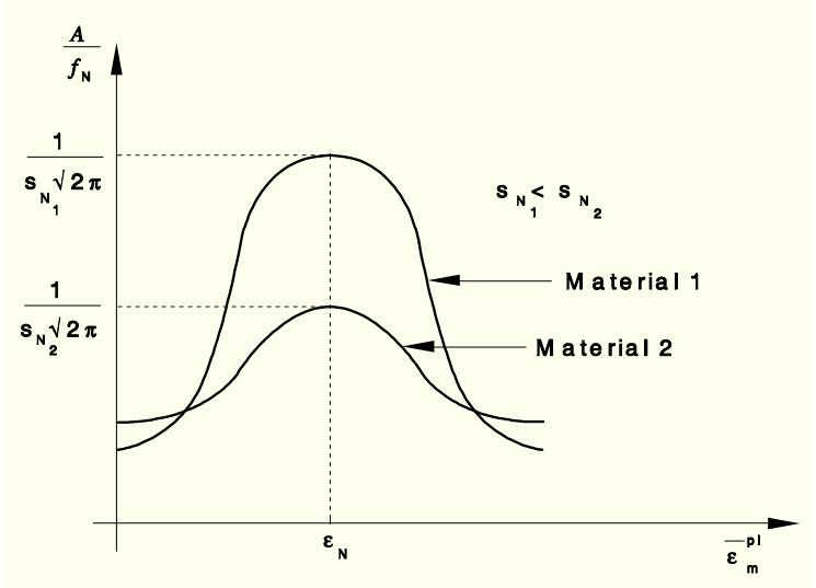ABAQUS assumes that the nucleation of new voids is plastic strain controlled (see Chu and Needleman, 1980), so that $$ \dot {f} _ {\mathrm{nucl}} = A \dot {\bar {\varepsilon}} _ {m} ^ {p l}, $$ where $$ A = \frac {f _ {N}}{s _ {N} \sqrt {2 \pi}} \exp \left[ - \frac {1}{2} \left(\frac {\bar {\varepsilon} _ {m} ^ {p l} - \varepsilon_ {N}}{s _ {N}}\right) ^ {2} \right]. $$ The normal distribution of the nucleation strain has a mean value $\varepsilon _ { N }$ , a standard deviation $s _ { N }$ , and nucleates voids with volume fraction $f _ { N }$ . The total rate of change of f is given as $$ \dot {f} = \dot {f} _ {\mathrm{gr}} + \dot {f} _ {\mathrm{nucl}}. $$ Voids are nucleated only in tension; ABAQUS will not consider the nucleation term at a material point if the stress state is compressive. The nucleation function $A / f _ { N }$ , which is assumed to have a normal distribution, is shown in Figure 4.3.6-3 for different values of the parameter $s _ { N }$ . Figure 4.3.6-4 shows the extent of softening in a uniaxial tension test of a porous material for different values of $f _ { N }$ . Figure 4.3.6-3 Nucleation function $A / f _ { N }$ . 

line

| Material | ε_m (s_N) | A/f_N (s_N) | | ---------- | --------- | ----------- | | Material 1 | ε_N | 1 | | Material 2 | ε_N | 1 |

Figure 4.3.6-4 Softening (in uniaxial tension) as a function of $f _ { N }$ .