On substituting Eq. (13.4.6) into Eq. (13.4.12) and using the fact that the nodal temperatures $\{ t \}$ are independent of the general coordinates x and y and can therefore be taken outside the integrals, we have $$ \begin{array}{l} \pi_ {h} = \frac {1}{2} \{t \} ^ {T} \iint_ {V} [ B ] ^ {T} [ D ] [ B ] d V \{t \} - \{t \} ^ {T} \iint_ {V} [ N ] ^ {T} Q d V \\ - \{t \} ^ {T} \iint_ {S _ {2}} [ N ] ^ {T} q ^ {*} d S + \frac {1}{2} \iint_ {S _ {3}} h [ \{t \} ^ {T} [ N ] ^ {T} [ N ] \{t \} \\ - \left(\{t \} ^ {T} [ N ] ^ {T} + [ N ] \{t \}\right) T _ {\infty} + T _ {\infty} ^ {2} ] d S \tag {13.4.13} \\ \end{array} $$ In Eq. (13.4.13), the minimization is most easily accomplished by explicitly writing the surface integral $S _ { 3 }$ with $\{ t \}$ left inside the integral as shown. On minimizing Eq. (13.4.13) with respect to ftg, we obtain $$ \begin{array}{l} \frac {\partial \pi_ {h}}{\partial \{t \}} = \iiint_ {V} [ B ] ^ {T} [ D ] [ B ] d V \{t \} - \iiint_ {V} [ N ] ^ {T} Q d V \\ - \iint_ {S _ {2}} [ N ] ^ {T} q ^ {*} d S + \iint_ {S _ {3}} h [ N ] ^ {T} [ N ] d S \{t \} \\ - \iint_ {S _ {3}} [ N ] ^ {T} h T _ {\infty} d S = 0 \tag {13.4.14} \\ \end{array} $$ where the last term $h T _ { \infty } ^ { 2 }$ in Eq. (13.4.13) is a constant that drops out while minimizing $\pi _ { h }$ . Simplifying Eq. (13.4.14), we obtain $$ \left[ \iint_ {V} [ B ] ^ {T} [ D ] [ B ] d V + \iint_ {S _ {3}} h [ N ] ^ {T} [ N ] d s \right] \{t \} = \{f _ {Q} \} + \{f _ {q} \} + \{f _ {h} \} \tag {13.4.15} $$ where the force matrices have been defined by $$ \left\{f _ {Q} \right\} = \iint_ {V} [ N ] ^ {T} Q d V \quad \left\{f _ {q} \right\} = \iint_ {S _ {2}} [ N ] ^ {T} q ^ {*} d S \tag {13.4.16} $$ $$ \left\{f _ {h} \right\} = \iint_ {S _ {3}} [ N ] ^ {T} h T _ {\infty} d S $$ In Eq. (13.4.16), the first term $\{ f _ { Q } \}$ (heat source positive, sink negative) is of the same form as the body-force term, and the second term $\{ f _ { q } \}$ (heat flux, positive into the surface) and third term $\{ f _ { h } \}$ (heat transfer or convection) are similar to surface tractions (distributed loading) in the stress analysis problem. You can observe this fact by comparing Eq. (13.4.16) with Eq. (6.2.46). Because we are formulating element equations of the form $\underline{f} = \underline{k}\underline{t}$ , we have the element conduction matrix\* for the heat-transfer problem given in Eq. (13.4.15) by $$ [ k ] = \iint_ {V} [ B ] ^ {T} [ D ] [ B ] d V + \iint_ {S _ {3}} h [ N ] ^ {T} [ N ] d S \tag {13.4.17} $$ where the first and second integrals in Eq. (13.4.17) are the contributions of conduction and convection, respectively. Using Eq. (13.4.17) in Eq. (13.4.15), for each element, we have $$ \{f \} = [ k ] \{t \} \tag {13.4.18} $$ Using the first term of Eq. (13.4.17), along with Eqs. (13.4.7) and (13.4.9), the conduction part of the $[k]$ matrix for the one-dimensional element becomes $$ \begin{array}{l} [ k _ {c} ] = \iiint_ {V} [ B ] ^ {T} [ D ] [ B ] d V = \int_ {0} ^ {L} \left\{ \begin{array}{c} - \frac {1}{L} \\ \frac {1}{L} \end{array} \right\} [ K _ {x x} ] \left[ \begin{array}{c c} - \frac {1}{L} & \frac {1}{L} \end{array} \right] A d x \\ = \frac {A K _ {x x}}{L ^ {2}} \int_ {0} ^ {L} \left[ \begin{array}{c c} 1 & - 1 \\ - 1 & 1 \end{array} \right] d x \tag {13.4.19} \\ \end{array} $$ or, finally, $$ [ k _ {c} ] = \frac {A K _ {x x}}{L} \left[ \begin{array}{c c} 1 & - 1 \\ - 1 & 1 \end{array} \right] \tag {13.4.20} $$ The convection part of the $[k]$ matrix becomes $$ [ k _ {h} ] = \iint_ {S _ {3}} h [ N ] ^ {T} [ N ] d S = h P \int_ {0} ^ {L} \left\{ \begin{array}{c} 1 - \frac {\hat {x}}{L} \\ \frac {\hat {x}}{L} \end{array} \right\} \left[ \begin{array}{c c} 1 - \frac {\hat {x}}{L} & \frac {\hat {x}}{L} \end{array} \right] d \hat {x} $$ or, on integrating, $$ [ k _ {h} ] = \frac {h P L}{6} \left[ \begin{array}{l l} 2 & 1 \\ 1 & 2 \end{array} \right] \tag {13.4.21} $$ where $$ d S = P d \hat {x} $$ and P is the perimeter of the element (assumed to be constant). Therefore, adding Eqs. (13.4.20) and (13.4.21), we find that the $[k]$ matrix is $$ [ k ] = \frac {A K _ {x x}}{L} \left[ \begin{array}{c c} 1 & - 1 \\ - 1 & 1 \end{array} \right] + \frac {h P L}{6} \left[ \begin{array}{c c} 2 & 1 \\ 1 & 2 \end{array} \right] \tag {13.4.22} $$ When h is zero on the boundary of an element, the second term on the right side of Eq. (13.4.22) (convection portion of $[ k ] )$ is zero. This corresponds, for instance, to an insulated boundary. The force matrix terms, on simplifying Eq. (13.4.16) and assuming $Q , q ^ { * }$ , and product $h T _ { \infty }$ to be constant are $$ \left\{f _ {Q} \right\} = \iiint_ {V} \left[ N \right] ^ {T} Q d V = Q A \int_ {0} ^ {L} \left\{ \begin{array}{c} 1 - \frac {\hat {x}}{L} \\ \frac {\hat {x}}{L} \end{array} \right\} d \hat {x} = \frac {Q A L}{2} \left\{ \begin{array}{l} 1 \\ 1 \end{array} \right\} \tag {13.4.23} $$ and $\{ f _ { q } \} = \int \limits _ { S _ { 2 } } q ^ { * } [ N ] ^ { T } d S = q ^ { * } P \int _ { 0 } ^ { L } \left\{ \begin{array} { c } { { 1 - \displaystyle \frac { \hat { x } } { L } } } \\ { { \displaystyle \frac { \hat { x } } { L } } } \end{array} \right\} d \hat { x } = \frac { q ^ { * } P L } { 2 } \left\{ \begin{array} { c } { { 1 } } \\ { { 1 } } \end{array} \right\}$ ð13:4:24Þ and $\{ f _ { h } \} = \int _ { S _ { 3 } } \int h T _ { \infty } [ N ] ^ { T } d S = \frac { h T _ { \infty } P L } { 2 } \left\{ \begin{array} { l } { 1 } \\ { 1 } \end{array} \right\}$ ð13:4:25Þ S3 Therefore, adding Eqs. (13.4.23)–(13.4.25), we obtain $$ \{f \} = \frac {Q A L + q ^ {*} P L + h T _ {\infty} P L}{2} \left\{ \begin{array}{l} 1 \\ 1 \end{array} \right\} \tag {13.4.26} $$ Equation (13.4.26) indicates that one-half of the assumed uniform heat source $Q$ goes to each node, one-half of the prescribed uniform heat flux $q ^ { * }$ ( positive $q ^ { * }$ enters the body) goes to each node, and one-half of the convection from the perimeter surface $h T _ { \infty }$ goes to each node of an element. 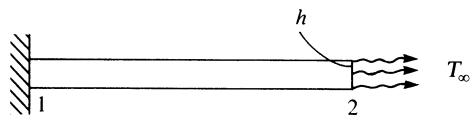Finally, we must consider the convection from the free end of an element. For simplicity’s sake, we will assume convection occurs only from the right end of the element, as shown in Figure 13–8. The additional convection term contribution to the stiffness matrix is given by $$ \left[ k _ {h} \right] _ {\text { end }} = \iint_ {S _ {\text { end }}} h [ N ] ^ {T} [ N ] d S \tag {13.4.27} $$ Now $N _ { 1 } = 0$ and $N _ { 2 } = 1$ at the right end of the element. Substituting the $N ^ { \prime } s$ into Eq. (13.4.27), we obtain $$ \left[ k _ {h} \right] _ {\text { end }} = \iint_ {S _ {\text { end }}} h \left\{ \begin{array}{l} 0 \\ 1 \end{array} \right\} [ 0 \quad 1 ] d S = h A \left[ \begin{array}{l l} 0 & 0 \\ 0 & 1 \end{array} \right] \tag {13.4.28} $$ 

text_image

1 h 2 T∞

Figure 13–8 Convection force from the end of an element The convection force from the free end of the element is obtained from the application of Eq. (13.4.25) with the shape functions now evaluated at the right end (where convection occurs) and with $S _ { 3 }$ (the surface over which convection occurs) now equal to the cross-sectional area A of the rod. Hence, $$ \{f _ {h} \} _ {\text { end }} = h T _ {\infty} A \left\{ \begin{array}{l} N _ {1} (\hat {x} = L) \\ N _ {2} (\hat {x} = L) \end{array} \right\} = h T _ {\infty} A \left\{ \begin{array}{l} 0 \\ 1 \end{array} \right\} \tag {13.4.29} $$ represents the convective force from the right end of an element where $N _ { 1 } ( \hat { x } = L )$ represents $N _ { 1 }$ evaluated at $\hat { x } = L$ , and so on. # Step 5 Assemble the Element Equations to Obtain the Global Equations and Introduce Boundary Conditions We obtain the global or total structure conduction matrix using the same procedure as for the structural problem (called the direct stiffness method as described in Section 2.4); that is, $$ [ K ] = \sum_ {e = 1} ^ {N} [ k ^ {(e)} ] \tag {13.4.30} $$ typically in units of $\mathrm { k W } / { } ^ { \circ } \mathrm { C }$ or $\mathrm { B t u / ( h \mathrm { - } ^ { \circ } F ) }$ . The global force matrix is the sum of all element heat sources and is given by $$ \{F \} = \sum_ {e = 1} ^ {N} \{f ^ {(e)} \} \tag {13.4.31} $$ typically in units of kW or Btu/h. The global equations are then $$ \{F \} = [ K ] \{t \} \tag {13.4.32} $$ with the prescribed nodal temperature boundary conditions given by Eq. (13.1.13). Note that the boundary conditions on heat flux, Eq. (13.1.11), and convection, Eq. (13.2.4), are actually accounted for in the same manner as distributed loading was accounted for in the stress analysis problem; that is, they are included in the column of force matrices through a consistent approach (using the same shape functions used to derive ½k ), as given by Eqs. (13.4.2). The heat-transfer problem is now amenable to solution by the finite element method. The procedure used for solution is similar to that for the stress analysis problem. In Section 13.5, we will derive the specific equations used to solve the twodimensional heat-transfer problem. # Step 6 Solve for the Nodal Temperatures We now solve for the global nodal temperature, ftg, where the appropriate nodal temperature boundary conditions, Eq. (13.1.13), are specified. # Step 7 Solve for the Element Temperature Gradients and Heat Fluxes Finally, we calculate the element temperature gradients from Eq. (13.4.6), and the heat fluxes, typically from Eq. (13.4.8). To illustrate the use of the equations developed in this section, we will now solve some one-dimensional heat-transfer problems. 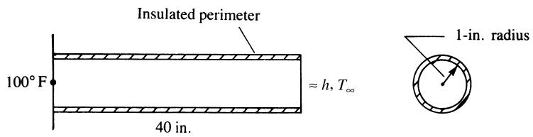# Example 13.1 Determine the temperature distribution along the length of the rod shown in Figure $_ { 1 3 - 9 }$ with an insulated perimeter. The temperature at the left end is a constant $1 0 0 ^ { \circ } \mathrm { F }$ and the free-stream temperature is $1 0 ^ { \circ } \mathrm { F }$ . Let $h = 1 0 \mathrm { \ B t u } / ( \mathrm { h } \mathrm { - f t } ^ { 2 } \mathrm { - } ^ { \circ } \mathrm { F } )$ and $K _ { x x } = 2 0 ~ \mathrm { B t u } / ( \mathrm { h } \mathrm { - f t } \mathrm { - } ^ { \circ } \mathrm { F } )$ . The value of h is typical for forced air convection and the value of $K _ { x x }$ is a typical conductivity for carbon steel (Tables 13–2 and 13–3). 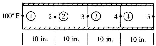The finite element discretization is shown in Figure 13–10. For simplicity’s sake, we will use four elements, each 10 in. long. There will be convective heat loss only over the right end of the rod because we consider the left end to have a known temperature and the perimeter to be insulated. We calculate the stiffness matrices for each element as follows: $$ \begin{array}{l} \frac {A K _ {x x}}{L} = \frac {\pi (1 \text {in.}) ^ {2} [ 2 0 \mathrm{Btu} / (\mathrm{h} - \mathrm{ft} - {} ^ {\circ} \mathrm{F}) ] (1 \mathrm{ft} ^ {2})}{\left(\frac {1 0 \text {in.}}{1 2 \text {in.} / \mathrm{ft}}\right) (1 4 4 \mathrm{in} ^ {2})} \\ = 0. 5 2 3 6 \mathrm{Btu} / (\mathrm{h} ^ {- \circ} \mathrm{F}) \\ \frac {h P L}{6} = \frac {\left[ 1 0 \mathrm{Btu} / \left(\mathrm{h} - \mathrm{ft} ^ {2} - ^ {\circ} \mathrm{F}\right) \right] (2 \pi)}{6} \left(\frac {1 \text {in.}}{1 2 \text {in. / ft}}\right) \left(\frac {1 0 \text {in.}}{1 2 \text {in. / ft}}\right) \tag {13.4.33} \\ = 0. 7 2 7 2 \mathrm{Btu} / (\mathrm{h} ^ {- \circ} \mathrm{F}) \\ h T _ {\infty} P L = \left[ 1 0 \mathrm{Btu} / \left(\mathrm{h} - \mathrm{ft} ^ {2} - ^ {\circ} \mathrm{F}\right) \right] \left(1 0 ^ {\circ} \mathrm{F}\right) (2 \pi) \left(\frac {1 \text {in.}}{1 2 \text {in.} / \mathrm{ft}}\right) \left(\frac {1 0 \text {in.}}{1 2 \text {in.} / \mathrm{ft}}\right) \\ = 4 3. 6 3 \mathrm{Btu} / \mathrm{h} \\ \end{array} $$ 

text_image

Insulated perimeter 100°F ≈ h, T∞ 40 in. 1-in. radius

Figure 13–9 One-dimensional rod subjected to temperature variation 

text_image

100° F ① 2 ② 3 ③ 4 ④ 5 10 in. 10 in. 10 in. 10 in.

Figure 13–10 Finite element discretized rod In general, from Eqs. (13.4.22) and (13.4.27), we have $$ [ k ] = \frac {A K _ {x x}}{L} \left[ \begin{array}{c c} 1 & - 1 \\ - 1 & 1 \end{array} \right] + \frac {h P L}{6} \left[ \begin{array}{c c} 2 & 1 \\ 1 & 2 \end{array} \right] + \iint_ {S _ {\text { end }}} h [ N ] ^ {T} [ N ] d S \tag {13.4.34} $$ Substituting Eqs. (13.4.33) into Eq. (13.4.34) for element 1, we have $$ [ k ^ {(1)} ] = 0. 5 2 3 6 \left[ \begin{array}{c c} 1 & - 1 \\ - 1 & 1 \end{array} \right] \mathrm{Btu} / (\mathrm{h} \cdot {} ^ {\circ} \mathrm{F}) \tag {13.4.35} $$ where the second and third terms on the right side of Eq. (13.4.34) are zero because there are no convection terms associated with element 1. Similarly, for elements 2 and 3, we have $$ [ k ^ {(2)} ] = [ k ^ {(3)} ] = [ k ^ {(1)} ] \tag {13.4.36} $$ However, element 4 has an additional (convection) term owing to heat loss from the flat surface at its right end. Hence, using Eq. (13.4.28), we have $$ \begin{array}{l} [ k ^ {(4)} ] = [ k ^ {(1)} ] + h A \left[ \begin{array}{c c} 0 & 0 \\ 0 & 1 \end{array} \right] \\ = 0. 5 2 3 6 \left[ \begin{array}{c c} 1 & - 1 \\ - 1 & 1 \end{array} \right] + [ 1 0 \mathrm{Btu} / (\mathrm{h} - \mathrm{ft} ^ {2} - ^ {\circ} \mathrm{F}) ] \pi \left(\frac {1 \text {in.}}{1 2 \text {in.} / \mathrm{ft}}\right) ^ {2} \left[ \begin{array}{c c} 0 & 0 \\ 0 & 1 \end{array} \right] \\ = \left[ \begin{array}{c c} 0. 5 2 3 6 & - 0. 5 2 3 6 \\ - 0. 5 2 3 6 & 0. 7 4 1 8 \end{array} \right] \mathrm{Btu} / (\mathrm{h} - ^ {\circ} \mathrm{F}) \tag {13.4.37} \\ \end{array} $$ In general, we would use Eqs. (13.4.23)-(13.4.25), and (13.4.29) to obtain the element force matrices. However, in this example, $Q = 0$ (no heat source), $q^{*} = 0$ (no heat flux), and there is no convection except from the right end. Therefore, $$ \{f ^ {(1)} \} = \{f ^ {(2)} \} = \{f ^ {(3)} \} = 0 \tag {13.4.38} $$ $$ \begin{array}{l} = [ 1 0 \mathrm{Btu} / (\mathrm{h} \cdot \mathrm{ft} ^ {2} \cdot {} ^ {\circ} \mathrm{F}) ] (1 0 ^ {\circ} \mathrm{F}) \pi \left(\frac {1 \text {in.}}{1 2 \text {in.} / \mathrm{ft}}\right) ^ {2} \left\{ \begin{array}{l} 0 \\ 1 \end{array} \right\} \\ = 2. 1 8 2 \left\{ \begin{array}{l} 0 \\ 1 \end{array} \right\} \mathrm{Btu} / \mathrm{h} \tag {13.4.39} \\ \end{array} $$ and $\{f^{(4)}\} = hT_{\infty}A\left\{ \begin{array}{l}0\\ 1 \end{array} \right\}$ The assembly of the element stiffness matrices [Eqs. (13.4.35)-(13.4.37)] and the element force matrices [Eqs. (13.4.38) and (13.4.39)], using the direct stiffness method, produces the following system of equations: $$ \left[ \begin{array}{c c c c c} 0. 5 2 3 6 & - 0. 5 2 3 6 & 0 & 0 & 0 \\ - 0. 5 2 3 6 & 1. 0 4 7 2 & - 0. 5 2 3 6 & 0 & 0 \\ 0 & - 0. 5 2 3 6 & 1. 0 4 7 2 & - 0. 5 2 3 6 & 0 \\ 0 & 0 & - 0. 5 2 3 6 & 1. 0 4 7 2 & - 0. 5 2 3 6 \\ 0 & 0 & 0 & - 0. 5 2 3 6 & 0. 7 4 1 8 \end{array} \right] \left\{ \begin{array}{l} t _ {1} \\ t _ {2} \\ t _ {3} \\ t _ {4} \\ t _ {5} \end{array} \right\} = \left\{ \begin{array}{l} F _ {1} \\ 0 \\ 0 \\ 0 \\ 2. 1 8 2 \end{array} \right\} \tag {13.4.40} $$ where $F _ { 1 }$ corresponds to an unknown rate of heat flow at node 1 (analogous to an unknown support force in the stress analysis problem). We have a known nodal temperature boundary condition of $t _ { 1 } = 1 0 0 ^ { \circ } \mathrm { F }$ . This nonhomogeneous boundary condition must be treated in the same manner as was described for the stress analysis problem (see Section 2.5 and Appendix B.4). We modify the stiffness (conduction) matrix and force matrix as follows: $$ \left[ \begin{array}{c c c c c} 1 & 0 & 0 & 0 & 0 \\ 0 & 1. 0 4 7 2 & - 0. 5 2 3 6 & 0 & 0 \\ 0 & - 0. 5 2 3 6 & 1. 0 4 7 2 & - 0. 5 2 3 6 & 0 \\ 0 & 0 & - 0. 5 2 3 6 & 1. 0 4 7 2 & - 0. 5 2 3 6 \\ 0 & 0 & 0 & - 0. 5 2 3 6 & 0. 7 4 1 8 \end{array} \right] \left\{ \begin{array}{l} t _ {1} \\ t _ {2} \\ t _ {3} \\ t _ {4} \\ t _ {5} \end{array} \right\} = \left\{ \begin{array}{c} 1 0 0 \\ 5 2. 3 6 \\ 0 \\ 0 \\ 2. 1 8 2 \end{array} \right\} \tag {13.4.41} $$ where the terms in the first row and column of the stiffness matrix corresponding to the known temperature condition, $t _ { 1 } = 1 0 0 ^ { \circ } \mathrm { F }$ , have been set equal to 0 except for the main diagonal, which has been set equal to 1, and the first row of the force matrix has been set equal to the known nodal temperature at node 1. Also, the term $( - 0 . 5 2 3 6 ) \times ( 1 0 0 ^ { \circ } \mathrm { F } ) = - 5 2 . 3 6$ on the left side of the second equation of Eq. (13.4.40) has been transposed to the right side in the second row $\left( \mathrm { a s } + 5 2 . 3 6 \right)$ of Eq. (13.4.41). The second through fifth equations of Eq. (13.4.41) corresponding to the rows of unknown nodal temperatures can now be solved (typically by Gaussian elimination). The resulting solution is given by $$ t _ {2} = 8 5. 9 3 ^ {\circ} \mathrm{F} \quad t _ {3} = 7 1. 8 7 ^ {\circ} \mathrm{F} \quad t _ {4} = 5 7. 8 1 ^ {\circ} \mathrm{F} \quad t _ {5} = 4 3. 7 5 ^ {\circ} \mathrm{F} \tag {13.4.42} $$ For this elementary problem, the closed-form solution of the differential equation for conduction, Eq. (13.1.9), with the left-end boundary condition given by Eq. (13.1.10) and the right-end boundary condition given by Eq. (13.2.4) yields a linear temperature distribution through the length of the rod. The evaluation of this linear temperature function at 10-in. intervals (corresponding to the nodal points used in the finite element model) yields the same temperatures as obtained in this example by the finite element method. Because the temperature function was assumed to be linear in each finite element, this comparison is as expected. Note that $F _ { 1 }$ could be determined by the first of Eqs. (13.4.40). 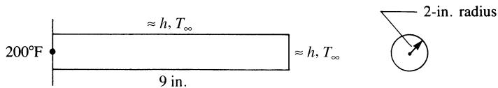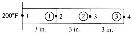# Example 13.2 To illustrate more fully the use of the equations developed in Section 13.4, we will now solve the heat-transfer problem shown in Figure 13–11. For the one-dimensional rod, determine the temperatures at 3-in. increments along the length of the rod and the rate of heat flow through element 1. Let $K _ { x x } = 3 ~ \mathrm { { B t u } / ( h – i n . \partial ^ { \circ } F ) , } h = 1 . 0 ~ \mathrm { { B t u } / ( h – i n ^ { 2 } \mathrm { { \circ } F ) } }$ , and $T _ { \infty } = 0 ^ { \circ } \mathrm { F }$ . The temperature at the left end of the rod is constant at $2 0 0 ^ { \circ } \mathrm { F }$ . The finite element discretization is shown in Figure 13–12. Three elements are sufficient to enable us to determine temperatures at the four points along the rod, although more elements would yield answers more closely approximating the analytical solution obtained by solving the differential equation such as Eq. (13.2.3) with the partial derivative with respect to time equal to zero. There will be convective heat loss over the perimeter and the right end of the rod. The left end will not have convective heat loss. Using Eqs. (13.4.22) and (13.4.28), we calculate the stiffness matrices for the elements as follows: $$ \frac {A K _ {x x}}{L} = \frac {(4 \pi) (3)}{3} = 4 \pi \mathrm{Btu} / (\mathrm{h} - ^ {\circ} \mathrm{F}) $$ $$ \frac {h P L}{6} = \frac {(1) (4 \pi) (3)}{6} = 2 \pi \mathrm{Btu} / (\mathrm{h} \cdot {} ^ {\circ} \mathrm{F}) \tag {13.4.43} $$ $$ h A = (1) (4 \pi) = 4 \pi \mathrm{Btu} / (\mathrm{h} - ^ {\circ} \mathrm{F}) $$ Substituting the results of Eqs. (13.4.43) into Eq. (13.4.22), we obtain the stiffness matrix for element 1 as $$ \begin{array}{l} [ k ^ {(1)} ] = 4 \pi \left[ \begin{array}{c c} 1 & - 1 \\ - 1 & 1 \end{array} \right] + 2 \pi \left[ \begin{array}{c c} 2 & 1 \\ 1 & 2 \end{array} \right] \\ = 4 \pi \left[ \begin{array}{c c} 2 & - \frac {1}{2} \\ - \frac {1}{2} & 2 \end{array} \right] \mathrm{Btu} / (\mathrm{h} \cdot {} ^ {\circ} \mathrm{F}) \tag {13.4.44} \\ \end{array} $$ Because there is no convection across the ends of element 1 (its left end has a known temperature and its right end is inside the whole rod and thus not exposed to fluid motion), the contribution to the stiffness matrix owing to convection from an end of the element, such as given by Eq. (13.4.28), is zero. Similarly, $$ [ k ^ {(2)} ] = [ k ^ {(1)} ] = 4 \pi \left[ \begin{array}{c c} 2 & - \frac {1}{2} \\ - \frac {1}{2} & 2 \end{array} \right] \mathrm{Btu} / (\mathrm{h} \cdot {} ^ {\circ} \mathrm{F}) \tag {13.4.45} $$ However, element 3 has an additional (convection) term owing to heat loss from the exposed surface at its right end. Therefore, Eq. (13.4.28) yields a contribution to the element 3 stiffness matrix, which is then given by $$ \begin{array}{l} [ k ^ {(3)} ] = [ k ^ {(1)} ] + h A \left[ \begin{array}{c c} 0 & 0 \\ 0 & 1 \end{array} \right] = 4 \pi \left[ \begin{array}{c c} 2 & - \frac {1}{2} \\ - \frac {1}{2} & 2 \end{array} \right] + 4 \pi \left[ \begin{array}{c c} 0 & 0 \\ 0 & 1 \end{array} \right] \\ = 4 \pi \left[ \begin{array}{c c} 2 & - \frac {1}{2} \\ - \frac {1}{2} & 3 \end{array} \right] \mathrm{Btu} / (\mathrm{h} \cdot {} ^ {\circ} \mathrm{F}) \tag {13.4.46} \\ \end{array} $$ 

text_image

200°F ≈ h, T∞ ≈ h, T∞ 9 in. 2-in. radius

Figure 13–11 One-dimensional rod subjected to temperature variation 

text_image

200°F 1 ① 2 ② 3 ③ 4 3 in. 3 in. 3 in.

Figure 13–12 Finite element discretized rod of Figure 13–11 In general, we calculate the force matrices by using Eqs. (13.4.26) and (13.4.29). Because $Q = 0 , q ^ { * } = 0 .$ , and $T _ { \infty } = 0 ^ { \circ } \mathrm { F }$ , all force terms are equal to zero. The assembly of the element matrices, Eqs. (13.4.44)–(13.4.46), using the direct stiffness method, produces the following system of equations: $$ 4 \pi \left[ \begin{array}{c c c c} 2 & - \frac {1}{2} & 0 & 0 \\ - \frac {1}{2} & 4 & - \frac {1}{2} & 0 \\ 0 & - \frac {1}{2} & 4 & - \frac {1}{2} \\ 0 & 0 & - \frac {1}{2} & 3 \end{array} \right] \left\{ \begin{array}{l} t _ {1} \\ t _ {2} \\ t _ {3} \\ t _ {4} \end{array} \right\} = \left\{ \begin{array}{l} F _ {1} \\ 0 \\ 0 \\ 0 \end{array} \right\} \tag {13.4.47} $$ We have a known nodal temperature boundary condition of $t _ { 1 } = 2 0 0 ^ { \circ } \mathrm { F }$ . As in Example 13.1, we modify the conduction matrix and force matrix as follows: $$ 4 \pi \left[ \begin{array}{c c c c} 1 & 0 & 0 & 0 \\ 0 & 4 & - \frac {1}{2} & 0 \\ 0 & - \frac {1}{2} & 4 & - \frac {1}{2} \\ 0 & 0 & - \frac {1}{2} & 3 \end{array} \right] \left\{ \begin{array}{l} t _ {1} \\ t _ {2} \\ t _ {3} \\ t _ {4} \end{array} \right\} = \left\{ \begin{array}{c} 8 0 0 \pi \\ 4 0 0 \pi \\ 0 \\ 0 \end{array} \right\} \tag {13.4.48} $$ where the terms in the first row and column of the conduction matrix corresponding to the known temperature condition, $t _ { 1 } = 2 0 0 ^ { \circ } \mathrm { F }$ , have been set equal to zero except for the main diagonal, which has been set to equal one, and the row of the force matrix has been set equal to the known nodal temperature at node 1. That is, the first row force is $( 2 0 0 ) ( 4 \pi ) = 8 0 0 \pi .$ , as we have left the 4p term as a multiplier of the elements inside the stiffness matrix. Also, the term $( - 1 / 2 ) ( 2 0 0 ) ( 4 \pi ) = - 4 0 0 \pi$ on the left side of the second equation of Eq. (13.4.47) has been transposed to the right side in the second row (as þ 400p) of Eq. (13.4.48). The second through fourth equations of Eq. (13.4.48), corresponding to the rows of unknown nodal temperatures, can now be solved. The resulting solution is given by $$ t _ {2} = 2 5. 4 ^ {\circ} \mathrm{F} \quad t _ {3} = 3. 2 4 ^ {\circ} \mathrm{F} \quad t _ {4} = 0. 5 4 ^ {\circ} \mathrm{F} \tag {13.4.49} $$ Next, we determine the heat flux for element 1 by using Eqs. (13.4.6) in (13.4.8) as $$ q ^ {(1)} = - K _ {x x} [ B ] \{t \} \tag {13.4.50} $$ Using Eq. (13.4.7) in Eq. (13.4.50), we have $$ q ^ {(1)} = - K _ {x x} \left[ - \frac {1}{L} \quad \frac {1}{L} \right] \left\{ \begin{array}{l} t _ {1} \\ t _ {2} \end{array} \right\} \tag {13.4.51} $$ Substituting the numerical values into Eq. (13.4.51), we obtain $$ q ^ {(1)} = - 3 \left[ - \frac {1}{3} \quad \frac {1}{3} \right] \left\{ \begin{array}{c} 2 0 0 \\ 2 5. 4 \end{array} \right\} $$ or $q ^ { ( 1 ) } = 1 7 4 . 6 \ \mathrm { B t u } / ( \mathrm { h } \mathrm { - i n } ^ { 2 } )$ ð13:4:52Þ We then determine the rate of heat flow $\bar { q }$ by multiplying Eq. (13.4.52) by the crosssectional area over which q acts. Therefore, $$ \bar {q} ^ {(1)} = 1 7 4. 6 (4 \pi) = 2 1 9 4 \mathrm{Btu/h} \tag {13.4.53} $$ Here positive heat flow indicates heat flow from node 1 to node 2 (to the right). # Example 13.3 The plane wall shown in Figure 13–13 is 1 m thick. The left surface of the wall $( x = 0 )$ is maintained at a constant temperature of $2 0 0 ^ { \circ } \mathrm { C } .$ , and the right surface $( x = L = 1 \mathrm { ~ m } )$ is insulated. The thermal conductivity is $K _ { x x } = 2 5 \ \mathrm { W } / ( \mathrm { m } \cdot { } ^ { \circ } \mathrm { C } )$ and there is a uniform generation of heat inside the wall of $Q = 4 0 0 \mathrm { W } / \mathrm { m } ^ { 3 }$ . Determine the temperature distribution through the wall thickness. 

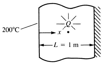
text_image

200°C x L = 1 m

Figure 13–13 Conduction in a plane wall subjected to uniform heat generation 

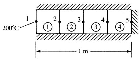
text_image

200°C 1 2 3 4 5 ① ② ③ ④ 1 m

Figure 13–14 Discretized model of Figure 13–13 This problem is assumed to be approximated as a one-dimensional heat-transfer problem. The discretized model of the wall is shown in Figure 13–14. For simplicity, we use four equal-length elements all with unit cross-sectional area $\left( A = 1 { \mathrm { m } } ^ { 2 } \right)$ . The unit area represents a typical cross section of the wall. The perimeter of the wall model is then insulated to obtain the correct conditions. Using Eqs. (13.4.22) and (13.4.28), we calculate the element stiffness matrices as follows: $$ \frac {A K _ {x x}}{L} = \frac {(1 \mathrm{m} ^ {2}) [ 2 5 \mathrm{W} / (\mathrm{m} \cdot {} ^ {\circ} \mathrm{C}) ]}{0 . 2 5 \mathrm{m}} = 1 0 0 \mathrm{W} / ^ {\circ} \mathrm{C} $$ For each identical element, we have $$ [ k ] = 1 0 0 \left[ \begin{array}{c c} 1 & - 1 \\ - 1 & 1 \end{array} \right] \mathrm{W} / ^ {\circ} \mathrm{C} \tag {13.4.54} $$ Because no convection occurs, h is equal to zero; therefore, there is no convection contribution to k. The element force matrices are given by Eq. (13.4.26). With $Q = 4 0 0 \mathrm { W } / \mathrm { m } ^ { 3 }$ , $q = 0 ;$ , and $h = 0 .$ , Eq. (13.4.26) becomes $$ \{f \} = \frac {Q A L}{2} \left\{ \begin{array}{l} 1 \\ 1 \end{array} \right\} \tag {13.4.55} $$ Evaluating Eq. (13.4.55) for a typical element, such as element 1, we obtain $$ \left\{ \begin{array}{l} f _ {1 x} \\ f _ {2 x} \end{array} \right\} = \frac {(4 0 0 \mathrm{W} / \mathrm{m} ^ {3}) (1 \mathrm{m} ^ {2}) (0 . 2 5 \mathrm{m})}{2} \left\{ \begin{array}{l} 1 \\ 1 \end{array} \right\} = \left\{ \begin{array}{l} 5 0 \\ 5 0 \end{array} \right\} \mathrm{W} \tag {13.4.56} $$ The force matrices for all other elements are equal to Eq. (13.4.56).