text_image

defined section anchor point 1 2 a Y anchor point elements used to define the section 2D and axisymmetric 3D 1 2 a Z Y X defined section

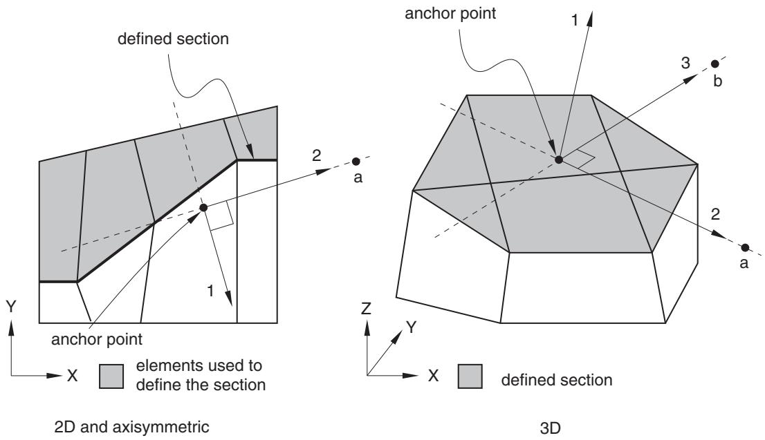
Figure 4.1.2–1 User-defined local coordinate system. the second (point b) must be in the local 2–3 plane on the side of the local 3-direction. Although it is not necessary, it is intuitive to select the second point such that it is on or near the local 3-direction (see Figure 4.1.2–1). If you do not specify the anchor point of the local system, it is taken to be the centroid of the projection of the surface on the fitted line or plane. If you do not specify the directions of the axes, the local system will be anchored at the specified anchor point and its axes will be parallel to the default axes of the projected surface. If neither the anchor point nor the directions are defined, the default local system will be used. In large-deformation analyses the surface section may rotate significantly during the deformation. By default, when output is requested in a local coordinate system, the system rotates with the average rigid body motion of the elements used to define the surface section (i.e., the local system and the output are updated during the analysis). The anchor point and local directions must then be specified relative to the undeformed configuration. You can choose to obtain vector output in the original local coordinate system instead. This choice is irrelevant in steps in which geometric nonlinearities are not considered. # Input File Usage: Use either of the following options to specify the local coordinate system directly: \*SECTION PRINT, NAME=section\_name, SURFACE=surface\_name, AXES=LOCAL, UPDATE=YES or NO anchor point definition axes definition ```python *SECTION FILE, NAME=section_name, SURFACE=surface_name, AXES=LOCAL, UPDATE=YES or NO anchor point definition axes definition ``` # Controlling the frequency of output You can control the frequency of section output by specifying the output frequency in increments. Unless a frequency of zero is specified to suppress output, the variables will always be output at the last increment of the step. Input File Usage: Use either of the following options: ```sql *SECTION PRINT, NAME=section_name, SURFACE=surface_name, FREQUENCY=n *SECTION FILE, NAME=section_name, SURFACE=surface_name, FREQUENCY=n ``` # Data file format Printed output is arranged in tables. The first line of the table contains the name of the requested output variable (see “Abaqus/Standard output variable identifiers,” Section 4.2.1), and the second line contains the corresponding value. If a section output request is defined without any specified output variables, all appropriate variables associated with the current analysis type are output. If several section output requests to the data file are encountered in one particular step, separate tables will be created for each request. Each table has a header denoting the name of the section and the name of the surface used. In addition, if the output is requested in a local coordinate system, the global coordinates of the anchor point and the cosine directions of the local axes are output. # Results file format Several section output records (record numbers 1580–1591 in “Results file output format,” Section 5.1.2) are output for each section output request to the results file. The actual collection of records to be written to the results file depends on the number of valid output requests. If a section output request is defined without any specified output variables, all records relevant to the current analysis type are stored in the results file. # Vector output in the section Vector output associated with section output requests consists of the total force (SOF), the total moment (SOM), and the center of forces (SOCF). Output variable SOF is computed as a vector sum of the stressbased (internal) nodal forces of the nodes in the surface. Output variable SOM is computed with respect to the origin of the coordinate system considered. Thus, if the output is requested in the global coordinate system, the total moment is computed about the global origin; if the output is requested in a local coordinate system, the moment is computed about the current anchor point of the local system. The coordinates of the current anchor point may change during the analysis if the local coordinate system is updated. Output variables SOF and SOM are both reported in the coordinate system considered. The center of forces SOCF is computed as the closest point to the centroid of the section through which the total force SOF acts. SOCF is always reported in the global coordinate system. If the total force vector is equal to zero, the centroid of the section is reported as the center of forces SOCF. The total moment vector, SOM, will not necessarily equal the cross product of the center of force vector, SOCF, and total force vector, SOF. Forces acting on two different points of the section may have components acting in opposite directions, such that these force components generate a net moment but not a net force; therefore, the total moment may not arise entirely from the resultant force. # Scalar output in the section Scalar output associated with a section output request consists of the area of the defined section (SOAREA), the total heat flux (SOH) in heat transfer analysis, the total current (SOE) in electrical analysis, the total mass flow (SOD) in mass diffusion analysis, and the total pore fluid volume flux (SOP) in couple pore fluid diffusion-stress analysis. These output variables are computed as the algebraic sum of the scalar internal nodal fluxes (work-conjugate to the associated primary solution variables) of the nodes in the surface. For example, in heat transfer analysis the total heat flux (SOH) is the sum of the NFLUX values at the nodes on the surfaces. # Limitations when using section output requests Section output requests are subject to the following limitations: • Section output requests are available only for sections defined by an element-based surface. Thus, they can be used only for sections along faces of continuum elements. • When defining the section, elements on only one side of the section must be used. Abaqus/Standard identifies all elements attached to the surface on this side and computes the section output variables as in a free-body diagram. 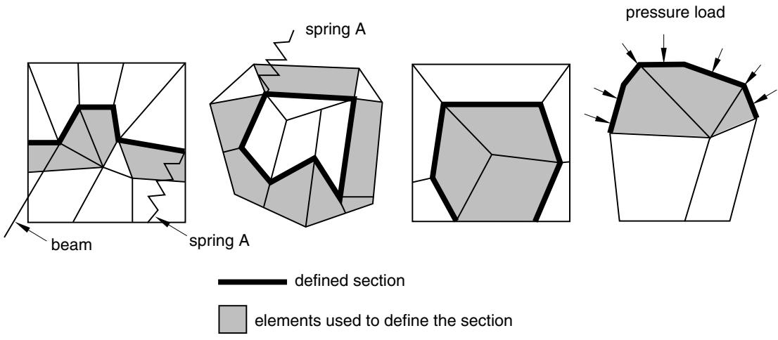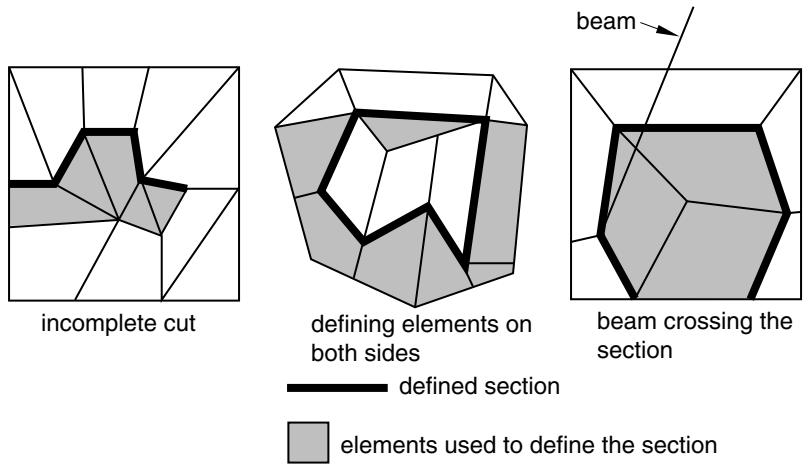• The defined section must cut completely through the mesh, form a closed surface, or be on the exterior of the body. Figure 4.1.2–2 presents some typical cases of valid surfaces. If the section cuts only partially through the mesh, a valid free-body diagram cannot be isolated (see Figure 4.1.2–3) and incorrect answers may be computed. Abaqus/Standard will attempt to identify the invalid cases and will issue error or warning messages. • Elements attached to the section can be on either side of the surface but must not cross the defined section. Figure 4.1.2–3 presents a few invalid cases. In most cases Abaqus/Standard will successfully identify elements that cross the surface, and warning messages will be issued. The elements will then not be considered in the calculation of the section variables. • For section output purposes, Abaqus/Standard will ignore the elements attached to the section for which it cannot establish whether they belong to one side or the other of the section (e.g., SPRING1 elements). • Section output requests cannot be specified within a substructure. • Section output requests cannot be specified in random response analyses. • The total force and the total moment in the section are computed based only on the stresses (internal forces) in the identified elements. Thus, inaccurate results may be obtained if distributed body 

text_image

beam spring A spring A pressure load defined section elements used to define the section

Figure 4.1.2–2 Valid section definitions. 

text_image

incomplete cut defining elements on both sides beam crossing the section defined section elements used to define the section

Figure 4.1.2–3 Invalid section definitions. loads are present in these elements since their effect on the total force in the section is not included. Common examples are the inertial loading in dynamic analyses, gravity loads, distributed body forces, and centrifugal loads. In these cases the total force in the section may depend on the choice of elements used to define the section as illustrated in Figure 4.1.2–4(a). Assuming that gravity loading is the only active load, the element stresses will be different in the two elements. Hence, if the same section is defined first using element 1 and then using element 2, different answers for the total force will be obtained. In a similar way the effects of any distributed body fluxes (heat, electrical, etc.) prescribed in the identified elements are not included.  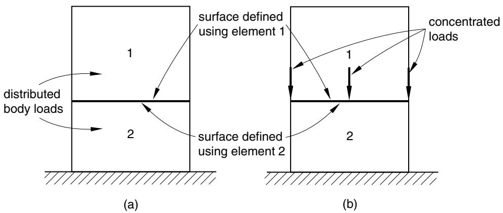Figure 4.1.2–4 Total force in the section. • Depending on which side of the surface is used to define the section, different answers will be obtained in analyses similar to the case illustrated in Figure 4.1.2–4(b). Assuming a static analysis with the concentrated loads shown in the figure being the only active loads, a zero total force is reported if the section is defined using element 1 and a nonzero force equal to the sum of the concentrated loads is obtained if the section is defined using element 2. # 4.1.3 OUTPUT TO THE OUTPUT DATABASE Products: Abaqus/Standard Abaqus/Explicit Abaqus/CFD Abaqus/CAE # References • “Element-based surface definition,” Section 2.3.2 • “Integrated output section definition,” Section 2.5.1 • “Output,” Section 4.1.1 • “The postprocessing calculator,” Section 4.3.1 • \*OUTPUT • \*FILTER • \*CONTACT OUTPUT • \*ELEMENT OUTPUT • \*ENERGY OUTPUT • \*INTEGRATED OUTPUT • \*INCREMENTATION OUTPUT • \*MODAL OUTPUT • \*NODE OUTPUT • \*RADIATION OUTPUT • \*SURFACE OUTPUT • “Understanding output requests,” Section 14.4 of the Abaqus/CAE User’s Guide # Overview Output variables are available for: • element integration points, element section points, whole elements, and element sets; • surfaces in Abaqus/Explicit and Abaqus/CFD; • integrated output sections in Abaqus/Explicit and Abaqus/Standard; • nodes; and • the whole model. All the output variables are defined in “Abaqus/Standard output variable identifiers,” Section 4.2.1, “Abaqus/Explicit output variable identifiers,” Section 4.2.2, and “Abaqus/CFD output variable identifiers,” Section 4.2.3. Model information and analysis results are stored in terms of an assembly of part instances (see “Defining an assembly,” Section 2.10.1). See the Abaqus Scripting User’s Guide for a description of how to use the Abaqus Scripting Interface or C++ to access an output database. Three types of information are stored in the output database in Abaqus/Standard and Abaqus/Explicit: “field” output, “history” output, and diagnostic information. In Abaqus/CFD four types of information are stored in the output database: nodal field output, surface field output, element history output, and surface history output. Field output and history output are controlled by output database requests as described in this section. A subset of the diagnostic information that is written to the message file for Abaqus/Standard analyses and to the status and message files for Abaqus/Explicit analyses is included in the output database. • Field output is intended for infrequent requests for a large portion of the model and can be used to generate contour plots, animations, symbol plots, X–Y plots, and displaced shape plots in Abaqus/CAE. Only complete sets of basic variables (for example, all the stress or strain components) can be requested as field output. • History output is intended for relatively frequent output requests for small portions of the model and is displayed in X–Y data plots in Abaqus/CAE. Individual variables (such as a particular stress component) can be requested. • Diagnostic information in Abaqus/Standard and Abaqus/Explicit is intended to provide analysis warning and/or error information as well as convergence information for use in Abaqus/CAE. Output database requests can be repeated as often as necessary within a step to produce both field and history output at multiple frequencies. # Requesting field output Contact surface output, element output, nodal output, and radiation output are available as field output in Abaqus/Standard and Abaqus/Explicit. Nodal, element, and surface output are available as field output in Abaqus/CFD. Input File Usage: Use the first option in conjunction with one or more of the subsequent options to request field output to the output database: \*OUTPUT, FIELD \*CONTACT OUTPUT \*ELEMENT OUTPUT \*NODE OUTPUT \*RADIATION OUTPUT \*SURFACE OUTPUT These options are discussed in detail below. Abaqus/CAE Usage: Step module: field output request editor # Requesting history output Contact surface output, element output, energy output, integrated output, time incrementation output, modal output, nodal output, and radiation output are available as history output in Abaqus/Standard and Abaqus/Explicit. Both element output and surface output are available as history output in Abaqus/CFD. Requesting large amounts of history output (more than 1000 output requests) may cause performance to degrade in Abaqus/Standard and will cause performance to degrade in Abaqus/Explicit and Abaqus/CFD. For vector- or tensor-valued output variables each component is considered to be a single request. In the case of element variables history output will be generated at each integration point. For example, requesting history output of the tensor variable S (stress) for a C3D10M element will generate 24 history output requests: (6 components) × (4 integration points). When requesting history output of vector- and tensor-valued variables, it is recommended that individual components be selected where available. Input File Usage: Use the first option in conjunction with one or more of the subsequent options to request history output to the output database: \*OUTPUT, HISTORY \*CONTACT OUTPUT \*ELEMENT OUTPUT \*ENERGY OUTPUT \*INTEGRATED OUTPUT \*INCREMENTATION OUTPUT \*MODAL OUTPUT \*NODE OUTPUT \*RADIATION OUTPUT \*SURFACE OUTPUT These options are discussed in detail below. Abaqus/CAE Usage: Step module: history output request editor # Requesting diagnostic information in Abaqus/Standard and Abaqus/Explicit By default, a subset of the diagnostic information that is written to the message file for Abaqus/Standard analyses and to the status and message files for Abaqus/Explicit analyses is also written to the output database. You can use the Visualization module of Abaqus/CAE to view this diagnostic information interactively, highlighting problematic areas on a view of the model and using them to resolve errors and warnings in the analysis. For more information, see “The message file in Abaqus/Standard and Abaqus/Explicit” in “Output,” Section 4.1.1, and Chapter 41, “Viewing diagnostic output,” of the Abaqus/CAE User’s Guide. Input File Usage: Use the following option to write diagnostic information to the output database: \*OUTPUT, DIAGNOSTICS=YES Use the following option to exclude diagnostic information: \*OUTPUT, DIAGNOSTICS=NO Abaqus/CAE Usage: You cannot exclude diagnostic information from the output database from within Abaqus/CAE. Use the following option to view the saved diagnostic information: Visualization module: Tools→Job Diagnostics The frequency of output to the output database is controlled differently in Abaqus/Standard, Abaqus/Explicit, and Abaqus/CFD. Control of the output frequency in Abaqus/Explicit depends upon whether field or history output was selected. # Controlling the output frequency in Abaqus/Standard Abaqus/Standard provides several options for controlling the output frequency, depending on whether the analysis is in the time domain (e.g., general statics), frequency domain (e.g., steady state dynamics), or mode domain (e.g., natural frequency extraction). These options can be used to reduce the amount of output written and hence improve performance and disk space use as compared to the default output. History output in Abaqus/Standard is buffered and is written to disk only after every 10 increments of history data output or when a step has completed. Therefore, history results may not be available immediately for postprocessing. # Default output frequency If you do not specify the output frequency, field and history output will be written at every increment of the analysis for all procedure types except dynamic and modal dynamic analyses for which output will be written every 10 increments. # Controlling output frequency in a frequency domain analysis In frequency domain procedures, you only can control the frequency of output by specifying the frequency of output in increments. The data will be written at this frequency as well as at the end of each step of the analysis. Specify an output frequency of zero to suppress output. Input File Usage: \*OUTPUT, FREQUENCY=n Abaqus/CAE Usage: Step module: field or history output request editor: Frequency: Every n increments: n # Controlling output frequency in a mode domain analysis In an eigenvalue extraction or eigenvalue buckling analysis, you can select the modes at which output is desired. If you do not specify a list of modes, output is produced for all of the modes. Input File Usage: \*OUTPUT, FIELD, MODE LIST Abaqus/CAE Usage: Step module: field output request editor: Frequency: Specify modes: list of modes # Controlling output frequency in a time domain analysis In time domain analyses, you can control the frequency of output by specifying the output frequency in terms of increments, the number of intervals during the step, the size of regular time intervals throughout the step, or time points throughout the step. The different options are described in more detail below.