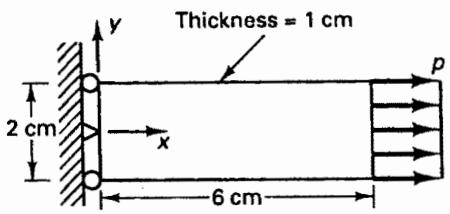
When using the load lumping procedure it should be recognized that the nodal point loads are, in general, calculated only approximately, and if a coarse finite element mesh is employed, the resulting solution may be very inaccurate. Indeed, in some cases when higher-order finite elements are used, surprising results are obtained. Figure 4.7 demonstrates such a case (see also Example 5.12). 

text_image

Thickness = 1 cm 2 cm x 6 cm y p

(a) Problem $$ \begin{array}{l} p = 3 0 0 \mathrm{N} / \mathrm{cm} ^ {2} \\ E = 3 \times 1 0 ^ {7} \mathrm{N} / \mathrm{cm} ^ {2} \\ \nu = 0. 3 \end{array} $$ 

text_image

y x A B C x p/3 4p/3 p/3

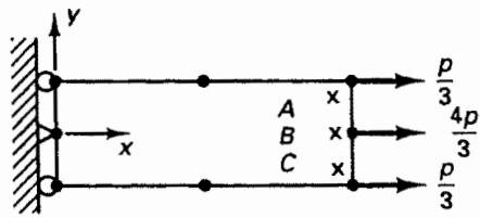
(b) Finite element model with consistent loading

Integration point	$\tau_{xx}$	$\tau_{yy}$	$\tau_{xy}$
A	300.00	0.0	0.0
B	300.00	0.0	0.0
C	300.00	0.0	0.0

(All stresses have units of N/cm²) 

text_image

y x A B C x p/2 p p/2

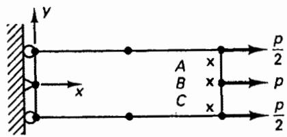
(c) Finite element model with lumped loading

Integration point	$\tau_{xx}$	$\tau_{yy}$	$\tau_{xy}$
A	301.41	-7.85	-24.72
B	295.74	-9.55	0.0
C	301.41	-7.85	24.72

(All stresses have units of N/cm²) (3 × 3 Gauss points are used, see Table 5.7) Figure 4.7 Some sample analysis results with and without consistent loading Considering dynamic analysis, the inertia effects can be thought of as body forces. Therefore, if a lumped mass matrix is employed, little might be gained by using a consistent load vector, whereas consistent nodal point loads should be used if a consistent mass matrix is employed in the analysis. 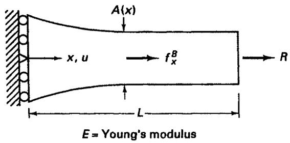# 4.2.5 Exercises 4.1. Use the procedure in Example 4.2 to formally derive the principle of virtual work for the one-dimensional bar shown. 

text_image

A(x) x, u f^B_x R L E = Young's modulus

The differential equations of equilibrium are $$ E \frac {\partial}{\partial x} \left(A \frac {\partial u}{\partial x}\right) + f _ {x} ^ {B} = 0 $$ $$ E A \left. \frac {\partial u}{\partial x} \right| _ {x = L} = R $$ 4.2. Consider the structure shown. (a) Write down the principle of virtual displacements by specializing the general equation (4.7) to this case. (b) Use the principle of virtual work to check whether the exact solution is $$ \tau (x) = \left(\frac {7 2}{7 3} + \frac {2 4 x}{7 3 L}\right) \frac {F}{A _ {0}} $$ Use the following three virtual displacements: (i) $\overline{u}(x) = a_0x$ , (ii) $\overline{u}(x) = a_0x^2$ , (iii) $\overline{u}(x) = a_0x^3$ . (c) Solve the governing differential equations of equilibrium, $$ E \frac {\partial}{\partial x} \left(A \frac {\partial u}{\partial x}\right) = 0 $$ $$ E A \left. \frac {\partial u}{\partial x} \right| _ {x = L} = F $$ (d) Use the three different virtual displacement patterns given in part (b), substitute into the principle of virtual work using the exact solution for the stress [from part (c)], and explicitly show that the principle holds. 

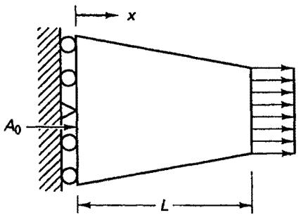
text_image

x A₀ L

F = total force exerted on right end $E =$ Young's modulus $A(x) = A_0(1 - x / 4L)$ # 4.3. Consider the bar shown. (a) Solve for the exact displacement response of the structure. (b) Show explicitly that the principle of virtual work is satisfied with the displacement patterns (i) $\overline{u} = ax$ and (ii) $\overline{u} = ax^2$ . (c) Identify a stress $\tau_{xx}$ for which the principle of virtual work is satisfied with pattern (ii) but not with pattern (i). 

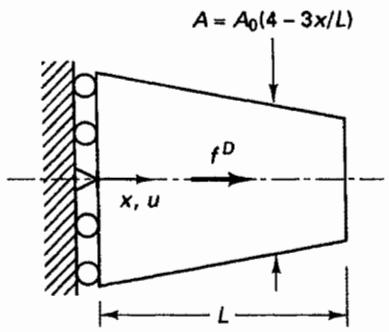
text_image

A = A₀(4 - 3x/L) f^D x, u L

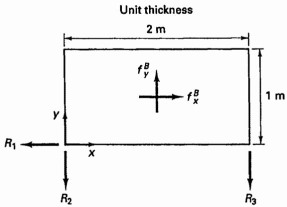
$f^{D}=$ constant force per unit length Young's modulus E 4.4. For the two-dimensional body shown, use the principle of virtual work to show that the body forces are in equilibrium with the applied concentrated nodal loads. $$ f _ {x} ^ {B} = 1 0 (1 + 2 x) \mathrm{N} / \mathrm{m} ^ {3} $$ $$ f _ {y} ^ {B} = 2 0 (1 + y) \mathrm{N} / \mathrm{m} ^ {3} $$ $$ R _ {1} = 6 0 \mathrm{N} $$ $$ R _ {2} = 4 5 \mathrm{N} $$ $$ R _ {3} = 1 5 \mathrm{N} $$ 

text_image

Unit thickness 2 m f_y^B f_x^B 1 m y x R_1 R_2 R_3

4.5. Idealize the bar structure shown as an assemblage of 2 two-node bar elements. (a) Calculate the equilibrium equations $\mathbf{K}\mathbf{U} = \mathbf{R}$ . (b) Calculate the mass matrix of the element assemblage. 

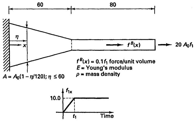
text_image

60 80 η x A = A₀(1 - η/120); η ≤ 60 f^B(x) → 20 A₀f₁ f^B(x) = 0.1f₁ force/unit volume E = Young's modulus ρ = mass density f₁ₓ 10.0 t₁ Time

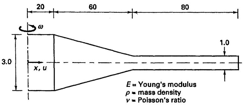
4.6. Consider the disk with a centerline hole of radius 20 shown spinning at a rotational velocity of $\omega$ radians/second. 

text_image

20 60 80 ω 3.0 x, u 1.0 E = Young's modulus ρ = mass density ν = Poisson's ratio

Idealize the structure as an assemblage of 2 two-node elements and calculate the steady-state (pseudostatic) equilibrium equations. (Note that the strains are now $\partial u/\partial x$ and u/x, where u/x is the hoop strain.) 4.7. Consider Example 4.5 and the state at time t = 2.0 with $U_{1}(t) = 0$ at all times. (a) Use the finite element formulation given in the example to calculate the static nodal point displacements and the element stresses. (b) Calculate the reaction at the support. (c) Let the calculated finite element solution be $u^{FE}$ . Calculate and plot the error r measured in satisfying the differential equation of equilibrium, i.e., $$ r = E \left[ \frac {\partial}{\partial x} \left(A \frac {\partial u ^ {\mathrm{FE}}}{\partial x}\right) \right] + f _ {x} ^ {B} A $$ (d) Calculate the strain energy of the structure as evaluated in the finite element solution and compare this strain energy with the exact strain energy of the mathematical model. 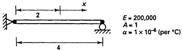4.8. The two-node truss element shown, originally at a uniform temperature, $20^{\circ}$ C, is subjected to a temperature variation $$ \theta = (1 0 x + 2 0) ^ {\circ} \mathrm{C} $$ Calculate the resulting stress and nodal point displacement. Also obtain the analytical solution, assuming a continuum, and briefly discuss your results. 

text_image

E = 200,000 A = 1 α = 1 × 10⁻⁶ (per °C)

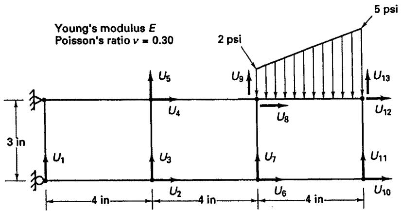
4.9. Consider the finite element analysis illustrated. 

other

| Position | U1 (in) | U2 (in) | U3 (in) | U4 (in) | U5 (in) | U6 (in) | U7 (in) | U8 (in) | U9 (in) | U10 (in) | U11 (in) | U12 (in) | U13 (in) | |----------|---------|---------|---------|---------|---------|---------|---------|---------|---------|----------|----------|----------|----------| | U1 | 3 | 4 | 4 | 4 | 4 | 4 | 4 | 4 | 4 | 4 | 4 | 4 | 4 | | U2 | 3 | 4 | 4 | 4 | 4 | 4 | 4 | 4 | 4 | 4 | 4 | 4 | 4 | | U3 | 3 | 4 | 4 | 4 | 4 | 4 | 4 | 4 | 4 | 4 | 4 | 4 | 4 | | U4 | 3 | 4 | 4 | 4 | 4 | 4 | 4 | 4 | 4 | 4 | 4 | 4 | 4 | | U5 | 3 | 4 | 4 | 4 | 4 | 4 | 4 | 4 | 4 | 4 | 4 | 4 | 4 | | U6 | 3 | 4 | 4 | 4 | 4 | 4 | 4 | 4 | 4 | 4 | 4 | 4 | 4 | | U7 | 3 | 4 | 4 | 4 | 4 | 4 | 4 | 4 | 4 | 4 | 4 | 4 | 4 | | U8 | 3 | 4 | 4 | 4 | 4 | 4 | 4 | 4 | 4 | 4 | 4 | 4 | 4 | | U9 | 3 | 4 | 4 | 4 | 4 | 4 | 4 | 4 | 4 | 4 | 4 | 4 | 4 | | U10 | 3 | 4 | 4 | 4 | 4 | 4 | 4 | 4 | 4 | 4 | 4 | 4 | 4 | | U11 | 3 | 4 | 4 | 4 | 4 | 4 | 4 | 4 | 4 | 4 | 4 | 4 | 4 | | U12 | 3 | 4 | 4 | 4 | 4 | 4 | 4 | 4 | 4 | 4 | 4 | 4 | 4 | | U13 | 3 | 4 | 4 | 4 | 4 | 4 | 4 | 4 | 4 | 4 | 4 | 4 | 4 |

Plane stress condition (thickness t). All elements are 4-node elements (a) Begin by establishing the typical matrix $\mathbf{B}$ of an element for the vector $\hat{\mathbf{u}}^T = [u_1 v_1 u_2 v_2 u_3 v_3 u_4 v_4]$ . (b) Calculate the elements of the K matrix, $K_{U_{2}U_{2}}$ , $K_{U_{6}U_{7}}$ , $K_{U_{7}U_{6}}$ , and $K_{U_{5}U_{12}}$ of the structural assemblage. (c) Calculate the nodal load $R_{9}$ due to the linearly varying surface pressure distribution. 

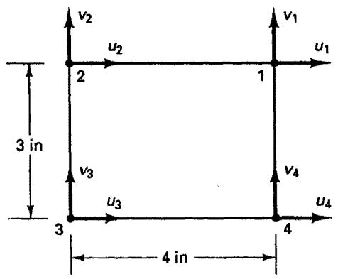
text_image

v2 u2 2 1 3 in v3 u3 3 4 in v1 u1 v4 u4

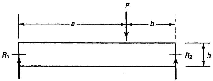
# 4.10. Consider the simply supported beam shown. (a) Assume that usual beam theory is employed and use the principle of virtual work to evaluate the reactions $R_{1}$ and $R_{2}$ . 

text_image

P a b R₁ R₂ h

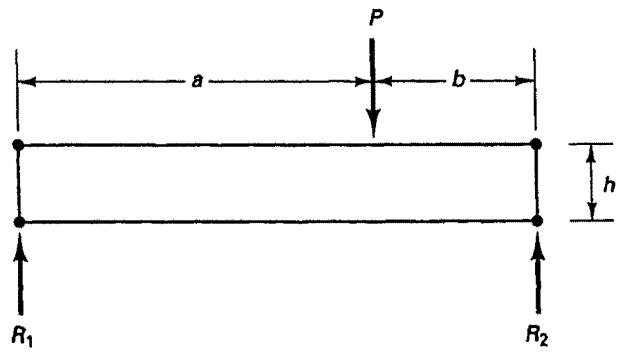
(b) Now assume that the beam is modeled by a four-node finite element. Show that to be able to evaluate $R_{1}$ and $R_{2}$ as in part (a) it is necessary that the finite element displacement functions can represent the rigid body mode displacements. 

text_image

P a b h R₁ R₂

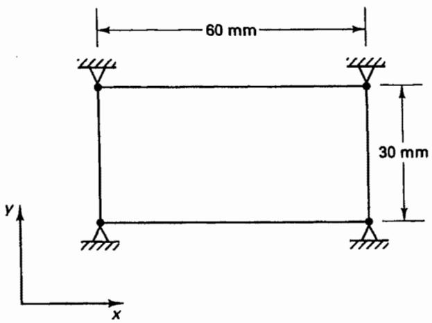
4.11. The four-node plane stress element shown carries the initial stresses $$ \tau_ {x x} ^ {I} = 0 \mathrm{MPa} $$ $$ \tau_ {y y} ^ {I} = 1 0 \mathrm{MPa} $$ $$ \tau_ {x y} ^ {I} = 2 0 \mathrm{MPa} $$ (a) Calculate the corresponding nodal point forces $R_{i}$ . (b) Evaluate the nodal point forces $\mathbf{R}_s$ equivalent to the surface tractions that correspond to the element stresses. Check your results using elementary statics and show that $\mathbf{R}_s$ is equal to $\mathbf{R}_l$ evaluated in part (a). Explain why this result makes sense. (c) Derive a general result: Assume that any stresses are given, and $R_{l}$ and $R_{s}$ are calculated. What conditions must the given stresses satisfy in order that $R_{l} = R_{s}$ , where the surface tractions in $R_{s}$ are obtained from equation (b) in Example 4.2? 

text_image

60 mm 30 mm y x

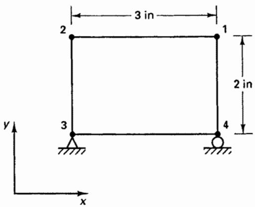
Young's modulus E Poisson's ratio v Thickness = 0.5 mm 4.12. The four-node plane strain element shown is subjected to the constant stresses $$ \tau_ {x x} = 2 0 \mathrm{psi} $$ $$ \tau_ {y y} = 1 0 \mathrm{psi} $$ $$ \tau_ {x y} = 1 0 \mathrm{psi} $$ Calculate the nodal point displacements of the element. 

text_image

3 in 2 1 2 in 3 4 y x

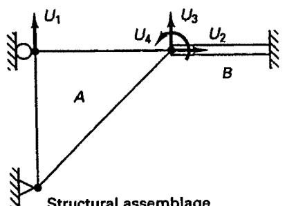
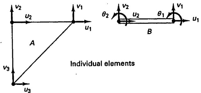
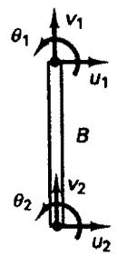
Young's modulus $E = 30 \times 10^{6}$ psi Poisson's ratio $\nu = 0.30$ 4.13. Consider element 2 in Fig. E4.9. (a) Show explicitly that $$ \mathbf {F} ^ {(2)} = \int_ {V ^ {(2)}} \mathbf {B} ^ {(2) T} \boldsymbol {\tau} ^ {(2)} d V ^ {(2)} $$ (b) Show that the element nodal point forces $\mathbf{F}^{(2)}$ are in equilibrium. 4.14. Assume that the element stiffness matrices $K_{A}$ and $K_{B}$ corresponding to the element displacements shown have been calculated. Assemble these element matrices directly into the global structure stiffness matrix with the displacement boundary conditions shown. 

text_image

U₁ U₄ U₃ U₂ A B Structural assemblage

Structural assemblage and degrees of freedom 

text_image

v2 u2 v1 u1 A v3 u3 θ2 v2 u2 θ1 v1 u1 B Individual elements

$$ \mathbf {K} _ {A} = \left[ \begin{array}{l l l l l l} a _ {1 1} & a _ {1 2} & a _ {1 3} & a _ {1 4} & a _ {1 5} & a _ {1 6} \\ a _ {2 1} & a _ {2 2} & a _ {2 3} & a _ {2 4} & a _ {2 5} & a _ {2 6} \\ a _ {3 1} & a _ {3 2} & a _ {3 3} & a _ {3 4} & a _ {3 5} & a _ {3 6} \\ a _ {4 1} & a _ {4 2} & a _ {4 3} & a _ {4 4} & a _ {4 5} & a _ {4 6} \\ a _ {5 1} & a _ {5 2} & a _ {5 3} & a _ {5 4} & a _ {5 5} & a _ {5 6} \\ a _ {6 1} & a _ {6 2} & a _ {6 3} & a _ {6 4} & a _ {6 5} & a _ {6 6} \end{array} \right] \left[ \begin{array}{l} u _ {1} \\ v _ {1} \\ u _ {2} \\ v _ {2} \\ u _ {3} \\ v _ {3} \end{array} \right] $$ $$ \mathbf {K} _ {B} = \left[ \begin{array}{l l l l l l} b _ {1 1} & b _ {1 2} & b _ {1 3} & b _ {1 4} & b _ {1 5} & b _ {1 6} \\ b _ {2 1} & b _ {2 2} & b _ {2 3} & b _ {2 4} & b _ {2 5} & b _ {2 6} \\ b _ {3 1} & b _ {3 2} & b _ {3 3} & b _ {3 4} & b _ {3 5} & b _ {3 6} \\ b _ {4 1} & b _ {4 2} & b _ {4 3} & b _ {4 4} & b _ {4 5} & b _ {4 6} \\ b _ {5 1} & b _ {5 2} & b _ {5 3} & b _ {5 4} & b _ {5 5} & b _ {5 6} \\ b _ {6 1} & b _ {6 2} & b _ {6 3} & b _ {6 4} & b _ {6 5} & b _ {6 6} \end{array} \right] \begin{array}{l} u _ {1} \\ v _ {1} \\ \theta_ {1} \\ u _ {2} \\ v _ {2} \\ \theta_ {2} \end{array} $$ 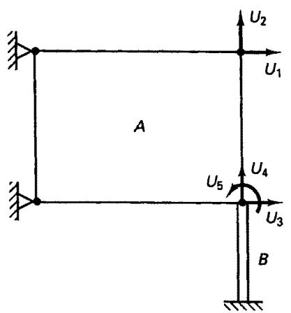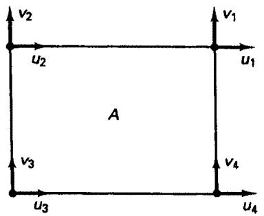4.15. Assume that the element stiffness matrices $K_{A}$ and $K_{B}$ corresponding to the element displacements shown have been calculated. Assemble these element matrices directly into the global structure stiffness matrix with the displacement boundary conditions shown. 

text_image

U2 U1 A U4 U5 U3 B

$$ \mathsf {K} _ {A} = \left[ \begin{array}{c c c c} a _ {1 1} & \ldots & \ldots & a _ {1 8} \\ \vdots & \ddots & & \vdots \\ \vdots & & \ddots & \vdots \\ a _ {8 1} & \ldots & \ldots & a _ {8 8} \end{array} \right] \begin{array}{l} u _ {1} \\ v _ {1} \\ u _ {2} \\ \vdots \\ v _ {4} \end{array} $$ $$ \mathbf {K} _ {B} = \left[ \begin{array}{c c c c} b _ {1 1} & \dots & \dots & b _ {1 6} \\ \vdots & \ddots & & \vdots \\ \vdots & & \ddots & \vdots \\ b _ {6 1} & \dots & \dots & b _ {6 6} \end{array} \right] \begin{array}{l} u _ {1} \\ v _ {1} \\ \theta_ {1} \\ \vdots \\ \theta_ {2} \end{array} $$ 

text_image

v₂ u₂ A v₁ u₁ v₃ u₃ v₄ u₄


text_image

θ₁ v₁ u₁ B θ₂ v₂ u₂

4.16. Consider Example 4.11. Assume that at the support $A$ , the roller allows a displacement only along a slope of 30 degrees to the horizontal direction. Determine the modifications necessary in the solution in Example 4.11 to obtain the structure matrix $\mathbf{K}$ for this situation. (a) Consider imposing the zero displacement condition exactly. (b) Consider imposing the zero displacement condition using the penalty method. 

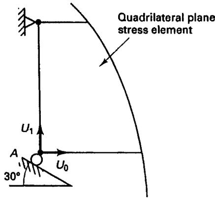
text_image

Quadrilateral plane stress element U₁ A 30° U₀

4.17. Consider the beam element shown. Evaluate the stiffness coefficients $k_{11}$ and $k_{12}$ . (a) Obtain the exact coefficients from the solution of the differential equation of equilibrium (using the mathematical model of Bernoulli beam theory). (b) Obtain the coefficients using the principle of virtual work with the Hermitian beam functions (see Example 4.16). 

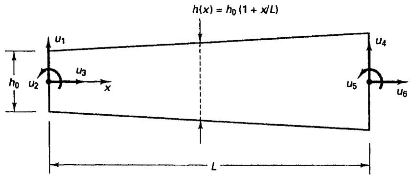
text_image

h(x) = h₀ (1 + x/L) u₁ u₃ u₂ x h₀ u₄ u₅ u₆ L

Young's modulus E Unit thickness 4.18. Consider the two-element assemblage shown. (a) Evaluate the stiffness coefficients $K_{11}$ , $K_{14}$ for the finite element idealization. (b) Calculate the load vector of the element assemblage. 

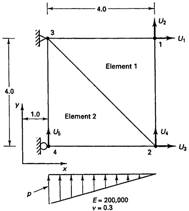
text_image

4.0 4.0 3 U2 U1 1 Element 1 Element 2 U5 4 U4 2 U3 x y 1.0 p E = 200,000 v = 0.3

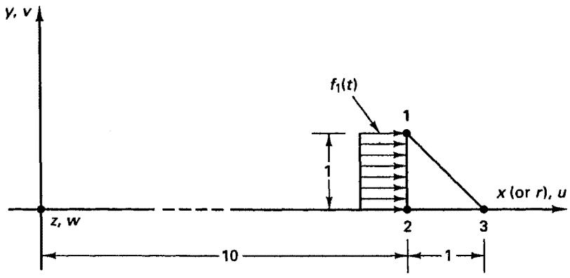
Plane stress, thickness = 0.1 4.19. Consider the two-element assemblage in Exercise 4.18 but now assume axisymmetric conditions. The $y$ -axis is the axis of revolution. (a) Evaluate the stiffness coefficients $K_{11}$ , $K_{14}$ for the finite element idealization. (b) Evaluate the corresponding load vector. 4.20. Consider Example 4.20 and let the loading on the structure be $R_r = f_1(t) \cos \theta$ . (a) Establish the stiffness matrix, mass matrix, and load vector of the three-node element 

text_image

y, v f₁(t) 1 z, w 10 2 1 3 x (or r), u

$$ E = 2 0 0, 0 0 0 $$ $$ \nu = 0. 3 $$ $$ \rho = \text { mass density } $$