flowchart

```mermaid graph TD A["Node 1"] --> B["Node 2"] B --> C["Node 3"] C --> D["Node 4"] D --> A ```


text_image

Nodes 2 and 3

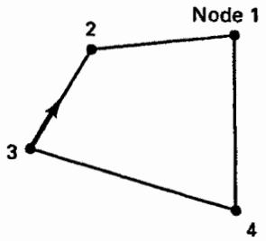
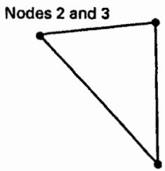
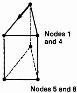
(a) Degeneration of 4-node to 3-node two-dimensional element 

text_image

Node 1 2 3 4 5 6 7 8


text_image

Nodes 5 and 8


text_image

Nodes 1 and 4 Nodes 5 and 8


flowchart

```mermaid graph TD A["Nodes 1 and 4"] --> B["Nodes 2 and 3"] A --> C["Nodes 5 and 8"] A --> D["Nodes 1 and 4"] A --> E["Nodes 2 and 3"] A --> F["Nodes 5 and 8"] ```


text_image

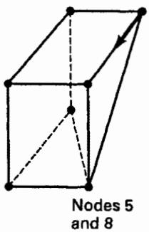
Nodes 1, 2, 3, and 4 Nodes 5 and 8

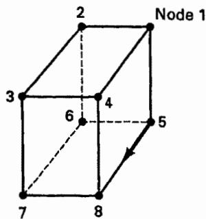
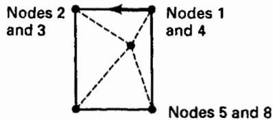
(b) Degenerate forms of 8-node three-dimensional element Figure 5.7 Degenerate forms of four- and eight-node elements of Figs. 5.4 and 5.5 EXAMPLE 5.15: Show that by collapsing the side 1-2 of the four-node quadrilateral element in Fig. E5.15 a constant strain triangle is obtained. Using the interpolation functions of Fig. 5.4, we have $$ x = \frac {1}{4} (1 + r) (1 + s) x _ {1} + \frac {1}{4} (1 - r) (1 + s) x _ {2} + \frac {1}{4} (1 - r) (1 - s) x _ {3} + \frac {1}{4} (1 + r) (1 - s) x _ {4} $$ $$ y = \frac {1}{4} (1 + r) (1 + s) y _ {1} + \frac {1}{4} (1 - r) (1 + s) y _ {2} + \frac {1}{4} (1 - r) (1 - s) y _ {3} + \frac {1}{4} (1 + r) (1 - s) y _ {4} $$ Thus, using the conditions $x_{1} = x_{2}$ and $y_{1} = y_{2}$ , we obtain $$ x = \frac {1}{2} (1 + s) x _ {2} + \frac {1}{4} (1 - r) (1 - s) x _ {3} + \frac {1}{4} (1 + r) (1 - s) x _ {4} $$ $$ y = \frac {1}{2} (1 + s) y _ {2} + \frac {1}{4} (1 - r) (1 - s) y _ {3} + \frac {1}{4} (1 + r) (1 - s) y _ {4} $$ 

text_image

y s 2 cm 1 r 3 4 x 2 cm y s 1,2 2 cm r 3 4 x 2 cm

Figure E5.15 Collapsing a plane stress four-node element to a triangular element and hence with the nodal coordinates given in Fig. E5.15, $$ x = \frac {1}{2} (1 + r) (1 - s) $$ $$ y = 1 + s $$ It follows that $$ \begin{array}{l} \frac {\partial x}{\partial r} = \frac {1}{2} (1 - s) \quad \frac {\partial y}{\partial r} = 0 \\ \frac {\partial x}{\partial s} = - \frac {1}{2} (1 + r) \quad \frac {\partial y}{\partial s} = 1 \end{array} ; \quad \mathbf {J} = \frac {1}{2} \left[ \begin{array}{c c} (1 - s) & 0 \\ - (1 + r) & 2 \end{array} \right]; \quad \mathbf {J} ^ {- 1} = \left[ \begin{array}{c c} \frac {2}{1 - s} & 0 \\ \frac {1 + r}{1 - s} & 1 \end{array} \right] $$ Using the isoparametric assumption, we also have $$ \begin{array}{l} u = \frac {1}{2} (1 + s) u _ {2} + \frac {1}{4} (1 - r) (1 - s) u _ {3} + \frac {1}{4} (1 + r) (1 - s) u _ {4} \\ v = \frac {1}{2} (1 + s) v _ {2} + \frac {1}{4} (1 - r) (1 - s) v _ {3} + \frac {1}{4} (1 + r) (1 - s) v _ {4} \\ \frac {\partial u}{\partial r} = - \frac {1}{4} (1 - s) u _ {3} + \frac {1}{4} (1 - s) u _ {4}; \quad \frac {\partial v}{\partial r} = - \frac {1}{4} (1 - s) v _ {3} + \frac {1}{4} (1 - s) v _ {4} \\ \frac {\partial u}{\partial s} = \frac {1}{2} u _ {2} - \frac {1}{4} (1 - r) u _ {3} - \frac {1}{4} (1 + r) u _ {4}; \quad \frac {\partial v}{\partial s} = \frac {1}{2} v _ {2} - \frac {1}{4} (1 - r) v _ {3} - \frac {1}{4} (1 + r) v _ {4} \\ \left[ \begin{array}{l} \frac {\partial}{\partial x} \\ \frac {\partial}{\partial y} \end{array} \right] = \mathbf {J} ^ {- 1} \left[ \begin{array}{l} \frac {\partial}{\partial r} \\ \frac {\partial}{\partial s} \end{array} \right] \\ \end{array} $$ Hence, $$ \left[ \begin{array}{l} \frac {\partial u}{\partial x} \\ \frac {\partial u}{\partial y} \end{array} \right] = \left[ \begin{array}{l l} \frac {2}{1 - s} & 0 \\ \frac {1 + r}{1 - s} & 1 \end{array} \right] \left[ \begin{array}{l l l l l l} 0 & 0 & - \frac {1}{4} (1 - s) & 0 & \frac {1}{4} (1 - s) & 0 \\ \frac {1}{2} & 0 & - \frac {1}{4} (1 - r) & 0 & - \frac {1}{4} (1 + r) & 0 \end{array} \right] \left[ \begin{array}{l} u _ {2} \\ v _ {2} \\ u _ {3} \\ v _ {3} \\ u _ {4} \\ v _ {4} \end{array} \right] $$ and $$ \left[ \begin{array}{l} \frac {\partial u}{\partial x} \\ \frac {\partial u}{\partial y} \end{array} \right] = \left[ \begin{array}{c c c c c c} 0 & 0 & - \frac {1}{2} & 0 & \frac {1}{2} & 0 \\ \frac {1}{2} & 0 & - \frac {1}{2} & 0 & 0 & 0 \end{array} \right] \left[ \begin{array}{l} u _ {2} \\ \vdots \\ u _ {4} \\ v _ {4} \end{array} \right] $$ Similarly, $$ \left[ \begin{array}{l} \frac {\partial v}{\partial x} \\ \frac {\partial v}{\partial y} \end{array} \right] = \left[ \begin{array}{l l l l l l} 0 & 0 & 0 & - \frac {1}{2} & 0 & \frac {1}{2} \\ 0 & \frac {1}{2} & 0 & - \frac {1}{2} & 0 & 0 \end{array} \right] \left[ \begin{array}{l} u _ {2} \\ \vdots \\ u _ {4} \\ v _ {4} \end{array} \right] $$ So we obtain $$ \epsilon = \left[ \begin{array}{c c c c c c} 0 & 0 & - \frac {1}{2} & 0 & \frac {1}{2} & 0 \\ 0 & \frac {1}{2} & 0 & - \frac {1}{2} & 0 & 0 \\ \frac {1}{2} & 0 & - \frac {1}{2} & - \frac {1}{2} & 0 & \frac {1}{2} \end{array} \right] \left[ \begin{array}{l} u _ {2} \\ v _ {2} \\ u _ {3} \\ v _ {3} \\ u _ {4} \\ v _ {4} \end{array} \right] $$ For any values of $u_{2}$ , $v_{2}$ , $u_{3}$ , $v_{3}$ , and $u_{4}$ , $v_{4}$ the strain vector is constant and independent of r, s. Thus, the triangular element is a constant strain triangle. In the preceding example we considered only one specific case. However, using the same approach it is apparent that collapsing any one side of a four-node plane stress or plane strain element will always result in a constant strain triangle. In considering the process of collapsing an element side, it is interesting to note that in the formulation used in Example 5.15 the matrix J is singular at $s = +1$ , but that this singularity disappears when the strain-displacement matrix is calculated. A practical consequence is that if in a computer program the general formulation of the four-node element is employed to generate a constant strain triangle (as in Example 5.15), the stresses should not be calculated at the two local nodes that have been assigned the same global node. 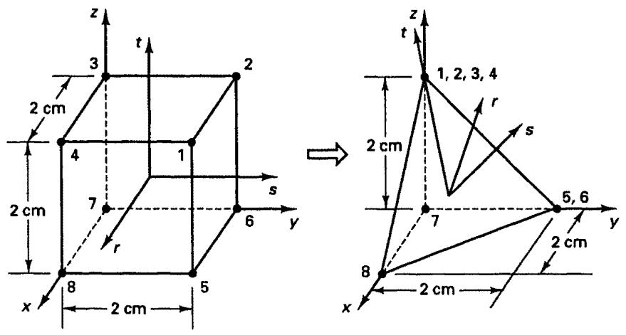(Since the stresses are constant throughout the element, they are conveniently evaluated at the center of the element, i.e., at r = 0, s = 0.) The same procedure can also be employed in three-dimensional analysis in order to obtain, from the basic eight-node element, wedge or tetrahedral elements. The procedure is illustrated in Fig. 5.7 and in the following example. EXAMPLE 5.16: Show that the three-dimensional tetrahedral element generated in Fig. E5.16 from the eight-node three-dimensional brick element is a constant strain element. Here we proceed as in Example 5.15. Thus, using the interpolation functions of the brick element (see Fig. 5.5) and substituting the nodal point coordinates of the tetrahedron, we obtain $$ x = \frac {1}{4} (1 + r) (1 - s) (1 - t) $$ $$ y = \frac {1}{2} (1 + s) (1 - t) $$ $$ z = 1 + t $$ 

text_image

z t 2 cm 3 2 4 1 2 cm 7 6 y x 2 cm 5 z t 1, 2, 3, 4 r s 2 cm 7 5, 6 y 2 cm 8 2 cm x

Figure E5.16 Collapsing an eight-node brick element into a tetrahedral element Hence, $$ \mathbf {J} = \left[ \begin{array}{c c c} \frac {1}{4} (1 - s) (1 - t) & 0 & 0 \\ - \frac {1}{4} (1 + r) (1 - t) & \frac {1}{2} (1 - t) & 0 \\ - \frac {1}{4} (1 + r) (1 - s) & - \frac {1}{2} (1 + s) & 1 \end{array} \right]; $$ $$ \mathbf {J} ^ {- 1} = \left[ \begin{array}{c c c} \frac {4}{(1 - s) (1 - t)} & 0 & 0 \\ \frac {2 (1 + r)}{(1 - s) (1 - t)} & \frac {2}{1 - t} & 0 \\ \frac {2 (1 + r)}{(1 - s) (1 - t)} & \frac {1 + s}{1 - t} & 1 \end{array} \right] \tag {a} $$ Using the same interpolation functions for u, and the conditions that $u_{1} = u_{2} = u_{3} = u_{4}$ and $u_{5} = u_{6}$ , we obtain $$ u = h _ {4} ^ {*} u _ {4} + h _ {5} ^ {*} u _ {5} + h _ {7} ^ {*} u _ {7} + h _ {8} ^ {*} u _ {8} $$ with $$ \begin{array}{l} h _ {4} ^ {*} = \frac {1}{2} (1 + t); \quad h _ {5} ^ {*} = \frac {1}{4} (1 + s) (1 - t); \\ h _ {7} ^ {*} = \frac {1}{8} (1 - r) (1 - s) (1 - t); \quad h _ {8} ^ {*} = \frac {1}{8} (1 + r) (1 - s) (1 - t) \\ \end{array} $$ Similarly, we also have $$ \begin{array}{l} v = h _ {4} ^ {*} v _ {4} + h _ {5} ^ {*} v _ {5} + h _ {7} ^ {*} v _ {7} + h _ {8} ^ {*} v _ {8} \\ w = h _ {4} ^ {*} w _ {4} + h _ {5} ^ {*} w _ {5} + h _ {7} ^ {*} w _ {7} + h _ {8} ^ {*} w _ {8} \\ \end{array} $$ Evaluating now the derivatives of the displacements $u, v,$ and $w$ with respect to $r, s,$ and $t,$ and using $\mathbf{J}^{-1}$ of (a), we obtain $$ \left[ \begin{array}{c} \frac {\partial u}{\partial x} \\ \frac {\partial v}{\partial y} \\ \frac {\partial w}{\partial z} \\ \frac {\partial u}{\partial y} + \frac {\partial v}{\partial x} \\ \frac {\partial v}{\partial z} + \frac {\partial w}{\partial y} \\ \frac {\partial u}{\partial z} + \frac {\partial w}{\partial x} \end{array} \right] = \left[ \begin{array}{c c c c c c c c c c c c c c c c} 0 & 0 & 0 & 0 & 0 & 0 & - \frac {1}{2} & 0 & 0 & \frac {1}{2} & 0 & 0 \\ 0 & 0 & 0 & 0 & \frac {1}{2} & 0 & 0 & - \frac {1}{2} & 0 & 0 & 0 & 0 \\ 0 & 0 & \frac {1}{2} & 0 & 0 & 0 & 0 & 0 & - \frac {1}{2} & 0 & 0 & 0 \\ 0 & 0 & 0 & \frac {1}{2} & 0 & 0 & - \frac {1}{2} & - \frac {1}{2} & 0 & 0 & \frac {1}{2} & 0 \\ 0 & \frac {1}{2} & 0 & 0 & 0 & \frac {1}{2} & 0 & - \frac {1}{2} & - \frac {1}{2} & 0 & 0 & 0 \\ \frac {1}{2} & 0 & 0 & 0 & 0 & 0 & - \frac {1}{2} & 0 & - \frac {1}{2} & 0 & 0 & \frac {1}{2} \end{array} \right] \left[ \begin{array}{c} u _ {4} \\ v _ {4} \\ w _ {4} \\ \dots \\ u _ {5} \\ v _ {5} \\ w _ {5} \\ \dots \\ u _ {7} \\ v _ {7} \\ w _ {7} \\ \dots \\ u _ {8} \\ v _ {8} \\ w _ {8} \end{array} \right] $$ Hence, the strains are constant for any nodal point displacements, which means that the element can represent only constant strain conditions. The process of collapsing an element side, or in three-dimensional analysis a number of element sides, may directly yield a desired element, but when higher-order two- or three-dimensional elements are employed, some special considerations may be necessary regarding the interpolation functions used. Specifically, when the lower-order elements displayed in Fig. 5.7 are employed, spatially isotropic triangular and wedge elements are automatically generated, but this is not necessarily the case when using higher-order elements. As an example, we consider the six-node triangular two-dimensional element obtained by collapsing one side of an eight-node element as shown in Fig. 5.8. If the triangular element has sides of equal length, we may want the element to be spatially isotropic; i.e., 

text_image

s 2 5 1 6 8 3 7 4 r Square element s 1, 2, 5 6 8 3 7 4 r Equilateral triangle

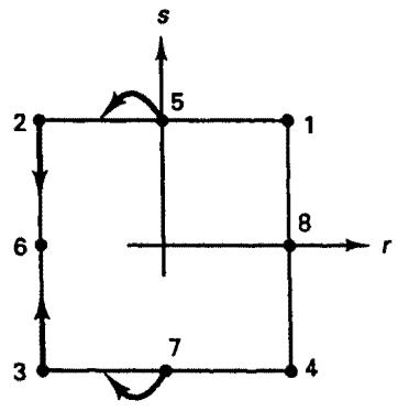
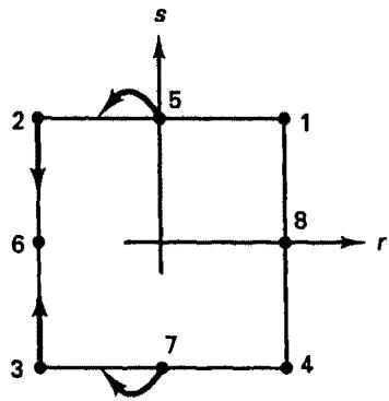
Figure 5.8 Collapsing an eight-node element into a triangle we may wish the internal element displacements u and v to vary in the same manner for each corner nodal displacement and each midside nodal displacement, respectively. However, the interpolation functions that are generated for the triangle when the side 1-2-5 of the square is simply collapsed do not fulfill the requirement that we should be able to change the numbering of the vertices without a change in the displacement assumptions. In order to fulfill this requirement, corrections need be applied to the interpolation functions of the nodes 3, 4, and 7 to obtain the final interpolations $h_{i}^{*}$ of the triangular element (see Exercise 5.25), $$ \begin{array}{l} h _ {1} ^ {*} = \frac {1}{2} (1 + s) - \frac {1}{2} (1 - s ^ {2}) \\ h _ {3} ^ {*} = \frac {1}{4} (1 - r) (1 - s) - \frac {1}{4} (1 - s ^ {2}) (1 - r) - \frac {1}{4} (1 - r ^ {2}) (1 - s) + \Delta h \\ h _ {4} ^ {*} = \frac {1}{4} (1 + r) (1 - s) - \frac {1}{4} (1 - r ^ {2}) (1 - s) - \frac {1}{4} (1 - s ^ {2}) (1 + r) + \Delta h \\ h _ {6} ^ {*} = \frac {1}{2} (1 - s ^ {2}) (1 - r) \tag {5.36} \\ h _ {7} ^ {*} = \frac {1}{2} (1 - r ^ {2}) (1 - s) - 2 \Delta h \\ h _ {8} ^ {*} = \frac {1}{2} (1 - s ^ {2}) (1 + r) \\ \end{array} $$ where we added the appropriate interpolations given in Fig. 5.4 and $$ \Delta h = \frac {(1 - r ^ {2}) (1 - s ^ {2})}{8} \tag {5.37} $$ Thus, to generate higher-order triangular elements by collapsing sides of square elements, it may be necessary to apply a correction to the interpolation functions used. 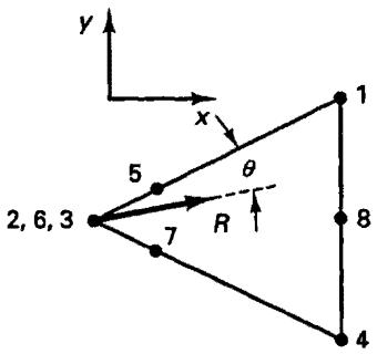# Triangular Elements in Fracture Mechanics In the preceding considerations, we assumed that a spatially isotropic element was desirable because the element was to be employed in a finite element assemblage used to predict a somewhat homogeneous stress field. However, in some cases, very specific stress variations are to be predicted, and in such analyses a spatially nonisotropic element may be more effective. One area of analysis in which specific spatially nonisotropic elements are employed is the field of fracture mechanics. Here it is known that specific stress singularities exist at crack tips, and for the calculation of stress intensity factors or limit loads, the use of finite elements that contain the required stress singularities can be effective. Various elements of this sort have been designed, but very simple and attractive elements can be obtained by distorting the higher-order isoparametric elements (see R. D. Henshell and K. G. Shaw [A] and R. S. Barsoum [A, B]). Figure 5.9 shows two-dimensional isoparametric elements that have been employed with much success in linear and nonlinear fracture mechanics because they contain the $1/\sqrt{R}$ and 1/R strain singularities, respectively. We should note that these elements have the interpolation functions given in (5.36) but with $\Delta h = 0$ . The same node-shifting and side-collapsing procedures can also be employed with higher-order three-dimensional elements in order to generate the required singularities. We demonstrate the procedure of node shifting to generate a strain singularity in the following example. 

flowchart

```mermaid graph TD 1["1"] -->|s| 5["5"] 5 -->|r| 8["8"] 8 --> 4["4"] 4 --> 7["7"] 7 --> 3["3"] 3 --> 6["6"] 6 --> 2["2"] 2 --> 1["1"] 1 --> 5 5 -->|s| 5 5 -->|r| 8 ```

Natural space Shift nodes 5 and 7 to quarter-points; collapse side 2-6-3 to one node 

text_image

y x 5 θ R 2, 6, 3 7 L/4 L 1 8 4

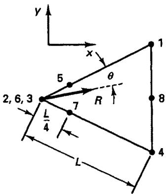
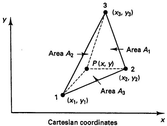
Actual physical space (a) Quarter-point triangular element with $1/\sqrt{R}$ strain singularity at node 2-6-3 

flowchart

```mermaid graph TD 1 -->|s| 5 5 -->|r| 8 8 --> 4 4 --> 7 7 --> 3 3 --> 6 6 --> 2 2 --> 1 ```

Natural space Shift nodes 5 and 7 to quarter-points; collapse side 2-6-3 but retain three nodes corresponding to 2, 6, and 3 

text_image

y x 5 θ 2, 6, 3 7 R 1 8 4

Actual physical space (b) Quarter-point triangular element with $1/\sqrt{R}$ and 1/R strain singularities at nodes 2, 6, and 3 Figure 5.9 Two-dimensional distorted (quarter point) isoparametric elements useful in fracture mechanics. Strain singularities are within the element for any angle $\theta$ . 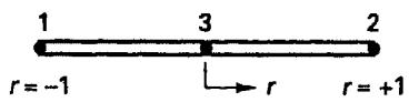[Note that in (a) the one node (2-6-3) has two degrees of freedom, and that in (b) nodes 2, 3, and 6 each have two degrees of freedom.] EXAMPLE 5.17: Consider the three-node truss element in Fig. E5.17. Show that when node 3 is specified to be at the quarter-point, the strain has a singularity of $1/\sqrt{x}$ at node 1. 

text_image

1 3 2 r = -1 → r r = +1

Natural space 

text_image

x 1 3 2 L/4 3L/4

Actual physical space Figure E5.17 Quarter-point one-dimensional element We have already considered a three-node truss in Example 5.2. Proceeding as before, we now have $$ x = \frac {r}{2} (1 + r) L + (1 - r ^ {2}) \frac {L}{4} $$ or $x = \frac{L}{4} (1 + r)^2$ (a) Hence, $\mathbf{J} = \left[\frac{L}{2} +\frac{r}{2} L\right]$ and the strain-displacement matrix is [using (b) in Example 5.2] $$ \mathbf {B} = \left[ \frac {1}{L / 2 + r L / 2} \right] \left[ \left(- \frac {1}{2} + r\right) \left(\frac {1}{2} + r\right) - 2 r \right] \tag {b} $$ To show the $1 / \sqrt{x}$ singularity we need to express $r$ in terms of $x$ . Using (a), we have $$ r = 2 \sqrt {\frac {x}{L}} - 1 $$ Substituting this value for $r$ into (b), we obtain $$ \mathbf {B} = \left[ \left(\frac {2}{L} - \frac {3}{2 \sqrt {L}} \frac {1}{\sqrt {x}}\right) \left(\frac {2}{L} - \frac {1}{2 \sqrt {L}} \frac {1}{\sqrt {x}}\right) \left(\frac {2}{\sqrt {L}} \frac {1}{\sqrt {x}} - \frac {4}{L}\right) \right] $$ Hence at $x = 0$ the quarter-point element in Fig. E5.17 has a strain singularity of order $1 / \sqrt{x}$ . 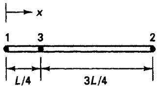# Triangular Elements by Area Coordinates Although the procedure of distorting a rectangular isoparametric element to generate a triangular element can be effective in some cases as discussed above, triangular elements (and in particular spatially isotropic elements) can be constructed directly by using area coordinates. For the triangle in Fig. 5.10, the position of a typical interior point P with coordinates x and y is defined by the area coordinates $$ L _ {1} = \frac {A _ {1}}{A}; \qquad L _ {2} = \frac {A _ {2}}{A}; \qquad L _ {3} = \frac {A _ {3}}{A} \tag {5.38} $$ 

text_image

3 (x₃, y₃) Area A₁ Area A₂ P (x, y) 2 (x₂, y₂) Area A₃ 1 (x₁, y₁) Cartesian coordinates x y


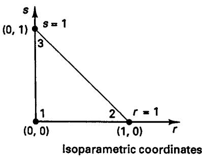
line

| Point | r | s | |---|---|---| | 1 | 0 | 1 | | 2 | 1 | 0 | | 3 | 1 | 0 | | s = 1 | 1 | 0 | | r = 1 | 1 | 0 | Isoparametric coordinates

Figure 5.10 Description of three-node triangle where the areas $A_{i}, i = 1, 2, 3$ , are defined in the figure and $A$ is the total area of the triangle. Thus, we also have $$ L _ {1} + L _ {2} + L _ {3} = 1 \tag {5.39} $$ Since element strains are obtained by taking derivatives with respect to the Cartesian coordinates, we need a relation that gives the area coordinates in terms of the coordinates $x$ and $y$ . Here we have $$ x = L _ {1} x _ {1} + L _ {2} x _ {2} + L _ {3} x _ {3} \tag {5.40} $$ $$ y = L _ {1} y _ {1} + L _ {2} y _ {2} + L _ {3} y _ {3} \tag {5.41} $$ because these relations hold at points 1, 2, and 3 and $x$ and $y$ vary linearly in between. Using (5.39) to (5.41), we have $$ \left[ \begin{array}{l} 1 \\ x \\ y \end{array} \right] = \left[ \begin{array}{l l l} 1 & 1 & 1 \\ x _ {1} & x _ {2} & x _ {3} \\ y _ {1} & y _ {2} & y _ {3} \end{array} \right] \left[ \begin{array}{l} L _ {1} \\ L _ {2} \\ L _ {3} \end{array} \right] \tag {5.42} $$ which gives $$ L _ {i} = \frac {1}{2 A} (a _ {i} + b _ {i} x + c _ {i} y); \quad i = 1, 2, 3 $$ where $2A = x_{1}y_{2} + x_{2}y_{3} + x_{3}y_{1} - y_{1}x_{2} - y_{2}x_{3} - y_{3}x_{1}$ $$ a _ {1} = x _ {2} y _ {3} - x _ {3} y _ {2}; \quad a _ {2} = x _ {3} y _ {1} - x _ {1} y _ {3}; \quad a _ {3} = x _ {1} y _ {2} - x _ {2} y _ {1} \tag {5.43} $$ $$ b _ {1} = y _ {2} - y _ {3}; \quad b _ {2} = y _ {3} - y _ {1}; \quad b _ {3} = y _ {1} - y _ {2} $$ $$ c _ {1} = x _ {3} - x _ {2}; \quad c _ {2} = x _ {1} - x _ {3}; \quad c _ {3} = x _ {2} - x _ {1} $$ As must have been expected, these $L_{i}$ are equal to the interpolation functions of a constant strain triangle. Thus, in summary we have for the three-node triangular element in Fig. 5.10, $$ u = \sum_ {i = 1} ^ {3} h _ {i} u _ {i}; \quad x \equiv \sum_ {i = 1} ^ {3} h _ {i} x _ {i} \tag {5.44} $$ $$ v = \sum_ {i = 1} ^ {3} h _ {i} v _ {i}; \quad y \equiv \sum_ {i = 1} ^ {3} h _ {i} y _ {i} $$ where $h_{i} = L_{i}, i = 1, 2, 3$ , and the $h_{i}$ are functions of the coordinates x and y. Using the relations in (5.44), the various finite element matrices of (5.27) to (5.35) can be directly evaluated. However, just as in the formulation of the quadrilateral elements (see Section 5.3.1), in practice, it is frequently expedient to use a natural coordinate space in order to describe the element coordinates and displacements. Using the natural coordinate system shown in Fig. 5.10, we have $$ h _ {1} = 1 - r - s; \quad h _ {2} = r; \quad h _ {3} = s \tag {5.45} $$ and the evaluation of the element matrices now involves a Jacobian transformation. Furthermore, all integrations are carried out over the natural coordinates; i.e., the r integrations go from 0 to 1 and the s integrations go from 0 to $(1 - r)$ . EXAMPLE 5.18: Using the isoparametric natural coordinate system in Fig. 5.10, establish the displacement and strain-displacement interpolation matrices of a three-node triangular element with $$ \begin{array}{l} x _ {1} = 0; \quad x _ {2} = 4; \quad x _ {3} = 1 \\ y _ {1} = 0; \quad y _ {2} = 0; \quad y _ {3} = 3 \\ \end{array} $$ In this case we have, using (5.44), $$ x = 4 r + s $$ $$ y = 3 s $$ Hence, using (5.23), $\mathbf{J} = \begin{bmatrix} 4 & 0 \\ 1 & 3 \end{bmatrix}$ and $\frac{\partial}{\partial\mathbf{x}} = \frac{1}{12}\left[ \begin{array}{cc}3 & 0\\ -1 & 4 \end{array} \right]\frac{\partial}{\partial\mathbf{r}}$ It follows that $$ \mathbf {H} = \left[ \begin{array}{c c c c c c c} (1 - r - s) & 0 & r & 0 & s & 0 \\ 0 & (1 - r - s) & 0 & r & 0 & s \end{array} \right] $$ and $\mathbf{B} = \frac{1}{12}\left[ \begin{array}{ccc:cc:cc} - 3 & 0 & & 3 & 0 & & 0 & 0\\ 0 & -3 & & 0 & -1 & & 0 & 4\\ -3 & -3 & & -1 & 3 & & 4 & 0 \end{array} \right]$ By analogy to the formulation of higher-order quadrilateral elements, we can also directly formulate higher-order triangular elements. Using the natural coordinate system in Fig. 5.10, which reduces to $$ L _ {1} = 1 - r - s; \quad L _ {2} = r; \quad L _ {3} = s \tag {5.46} $$ where the $L_{i}$ are the area coordinates of the “unit triangle,” the interpolation functions of a 3 to 6 variable-number-nodes element are given in Fig. 5.11. These functions are constructed in the usual way, namely, $h_{i}$ must be unity at node i and zero at all other nodes (see Example 5.1). $^{2}$ The interpolation functions of still higher-order triangular elements are obtained in a similar manner. Then the “cubic bubble function” $L_{1}L_{2}L_{3}$ is also employed. Using this approach we can now also directly construct the interpolation functions of three-dimensional tetrahedral elements. First, we note that in analogy to (5.46) we now employ volume coordinates $$ L _ {1} = 1 - r - s - t; \quad L _ {2} = r \tag {5.47} $$ $$ L _ {3} = s; \quad L _ {4} = t $$ where we may check that $L_{1} + L_{2} + L_{3} + L_{4} = 1$ . The $L_{i}$ in (5.47) are the interpolation functions of the four-node element in Fig. 5.12 in its natural space. The interpolation