text_image

x3 x2 x1 x2 x3 P(tx1, tx2, tx3) δu t u Time t P(0x1, 0x2, 0x3) Time 0 dashed line shows δu imposed onto configuration at time t

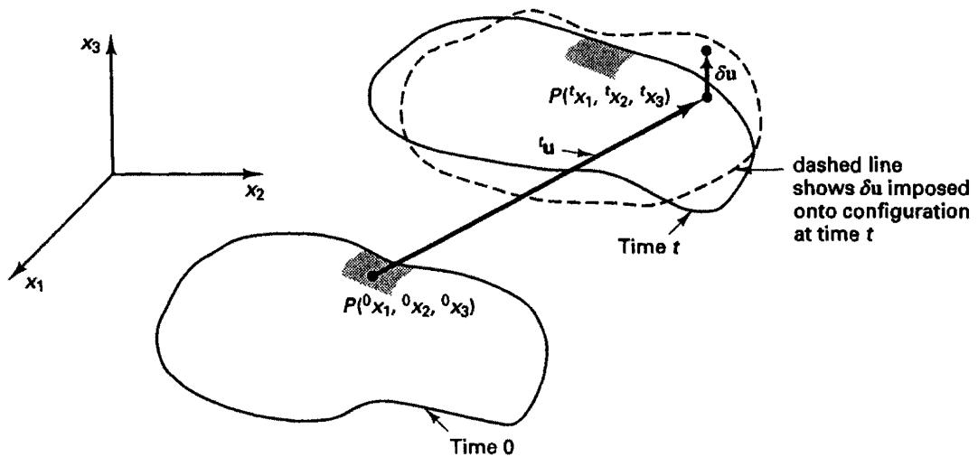
Figure E6.10 Body at time t subjected to virtual displacement field given by $\delta u$ . Note that $\delta u$ is a function of $^{t}x_{i}, i = 1,2,3$ , and we can think of $\delta u_{i}$ as a variation on $^{t}u_{i}$ . where $$ \delta_ {t} e _ {m n} = \frac {1}{2} \left(\frac {\partial \delta u _ {m}}{\partial^ {t} x _ {n}} + \frac {\partial \delta u _ {n}}{\partial^ {t} x _ {m}}\right) $$ We use the definition of the Green-Lagrange strain in (6.54) to obtain $$ \delta_ {0} ^ {\prime} \epsilon = \frac {1}{2} \left[ \left(\delta_ {0} ^ {\prime} \mathbf {X} ^ {T}\right) \left(_ {0} ^ {\prime} \mathbf {X}\right) + \left(_ {0} ^ {\prime} \mathbf {X} ^ {T}\right) \left(\delta_ {0} ^ {\prime} \mathbf {X}\right) \right] \tag {b} $$ Let us define $\delta_{i}\mathbf{u}$ to be $$ \delta_ {t} \mathbf {u} = \left[ \begin{array}{c c c} \frac {\partial \delta u _ {1}}{\partial^ {t} x _ {1}} & \frac {\partial \delta u _ {1}}{\partial^ {t} x _ {2}} & \dots \\ \frac {\partial \delta u _ {2}}{\partial^ {t} x _ {1}} & \frac {\partial \delta u _ {2}}{\partial^ {t} x _ {2}} & \dots \\ & \dots \end{array} \right] $$ then $$ \delta_ {0} ^ {t} \mathbf {X} = \delta_ {t} \mathbf {u} _ {0} ^ {t} \mathbf {X} $$ and hence (b) can be written as $$ \begin{array}{l} \delta_ {0} ^ {\prime} \epsilon = \frac {1}{2} \left[ _ {0} ^ {\prime} \mathbf {X} ^ {T} \left(\delta_ {t} \mathbf {u}\right) ^ {T} _ {0} ^ {\prime} \mathbf {X} + _ {0} ^ {\prime} \mathbf {X} ^ {T} \left(\delta_ {t} \mathbf {u}\right) _ {0} ^ {\prime} \mathbf {X} \right] \\ = _ {0} ^ {t} \mathbf {X} ^ {T} \left\{\frac {1}{2} \left[ \left(\delta_ {t} \mathbf {u}\right) ^ {T} + \delta_ {t} \mathbf {u} \right] \right\} _ {0} ^ {t} \mathbf {X} \\ = _ {0} ^ {t} \mathbf {X} ^ {T} \delta_ {t} \mathbf {e} _ {0} ^ {t} \mathbf {X} \\ \end{array} $$ which is (a) in matrix form. Note that a simple closed-form relationship cannot be established between the time rate of change of the Hencky strain tensor and the velocity strain tensor [because of the complex expression in (6.61)]. We shall use the Hencky strain measure only later for large strain inelastic analysis, and the appropriate relationships will then be evaluated based on work conjugacy (see Section 6.6.4). However, we shall use the Green-Lagrange strain tensor frequently and now want to define the appropriate stress tensor to use with this strain tensor. The stress measure to use is the second Piola-Kirchhoff stress tensor $\delta S$ , which is work-conjugate with the Green-Lagrange strain tensor. $^{4}$ Consider the stress power per unit reference volume $J^{\prime} \tau \cdot {}^{\prime} \mathbf{D}$ , where ${}^{\prime} \tau$ is the Cauchy stress tensor and $J = \det {}_{0}^{t} \mathbf{X}$ . Then the second Piola-Kirchhoff stress tensor ${}_{0}^{t} \mathbf{S}$ is given by $$ { } ^ { \prime } J { } ^ { \prime } \mathbf { T } \cdot { } ^ { \prime } \mathbf { D } = { } _ { 0 } ^ { \prime } \mathbf { S } \cdot { } _ { 0 } ^ { \prime } \dot { \boldsymbol { \epsilon } } \tag {6.66} $$ To find the explicit expression for $\delta S$ , we substitute from (6.63) to obtain $$ ^ \prime J ^ {\prime} \boldsymbol {\tau} \cdot {} ^ {\prime} \mathbf {D} = _ {0} ^ {\prime} \mathbf {S} \cdot (_ {0} ^ {\prime} \mathbf {X} ^ {T} {} ^ {\prime} \mathbf {D} _ {0} ^ {\prime} \mathbf {X}) \tag {6.67} $$ Since this relationship must hold for any 'D, we have $^{6}$ $$ \boxed { \begin{array}{c} \delta_ {0} ^ {t} \mathbf {S} = \frac {{} ^ {0} \rho}{t \rho} _ {t} ^ {0} \mathbf {X} ^ {t} \boldsymbol {\tau} _ {t} ^ {0} \mathbf {X} ^ {T} \end{array} } $$ (as a "pull-back") (6.68) $$ \boxed { \begin{array}{c} ^ {t} \boldsymbol {\tau} = \frac {^ {t} \rho}{^ {0} \rho} _ {0} ^ {t} \mathbf {X} _ {0} ^ {t} \mathbf {S} _ {0} ^ {t} \mathbf {X} ^ {T} \end{array} } $$ (as a "push-forward") or in component forms $$ \boxed { \begin{array}{c} _ {0} ^ {t} S _ {i j} = \frac {{} ^ {0} \rho}{^ {t} \rho} _ {i} ^ {0} x _ {i, m} ^ {0} x _ {j, n} ^ {^ {\prime}} \tau_ {m n} \end{array} } $$ (6.69) $$ \boxed { \begin{array}{c} ^ {\prime} \tau_ {m n} = \frac {^ {\prime} \rho}{^ {0} \rho} _ {0} ^ {\prime} x ^ {\prime} x ^ {\prime} S _ {i j} \end{array} } $$ There has been much discussion about the physical nature of the second Piola-Kirchhoff stress tensor. However, although it is possible to relate the transformation on the Cauchy stress tensor in $(6.68)$ to some geometry arguments as discussed in the next example, it should be recognized that the second Piola-Kirchhoff stresses have little physical meaning and, in practice, Cauchy stresses must be calculated. 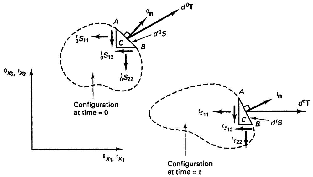EXAMPLE 6.11: Figure E6.11 shows a generic body in the configurations at times 0 and t. Let $d^{t}T$ be the actual force on a surface area $d^{t}S$ in the configuration at time t, and let us define a (fictitious) force $$ d ^ {0} \mathbf {T} = _ {t} ^ {0} \mathbf {X} d ^ {t} \mathbf {T}; \quad {} _ {t} ^ {0} \mathbf {X} = \left[ \frac {\partial^ {0} x _ {i}}{\partial^ {t} x _ {j}} \right] \tag {a} $$ which acts on the surface area $d^{0}S$ , where $d^{0}S$ has become $d^{\prime}S$ and ${}^{0}X$ is the inverse of the deformation gradient, ${}^{0}X = {}^{0}X^{-1}$ . Show that the second Piola-Kirchhoff stresses measured in the original configuration are the stress components corresponding to $d^{0}T$ . Let the unit normals to the surface areas $d^{0}S$ and $d'S$ be $^{0}n$ and $^{1}n$ , respectively. Force equilibrium (of the wedge ABC in Fig. E6.11) in the configuration at time t requires that $$ d ^ {t} \mathbf {T} = ^ {t} \boldsymbol {\tau} ^ {T} {} ^ {t} \mathbf {n} d ^ {t} S \tag {b} $$ and similarly in the configuration at time 0 $$ d ^ {0} \mathbf {T} = \mathbf {\delta} _ {0} \mathbf {S} ^ {T} {} ^ {0} \mathbf {n} d ^ {0} S \tag {c} $$ The relations in (b) and (c) are referred to as Cauchy's formula. However, it can be shown that the following kinematic relationship exists: $$ { } ^ { t } \mathbf { n } d ^ { t } S = \frac { { } ^ { 0 } \rho } { { } ^ { t } \rho } { } ^ { 0 } \mathbf { X } ^ { T } { } ^ { 0 } \mathbf { n } d ^ { 0 } S \tag {d} $$ This relation is referred to as Nanson's formula. Now using (a) to (d), we obtain $$ { } _ { 0 } ^ { t } \mathbf { S } ^ { T } { } ^ { 0 } \mathbf { n } d ^ { 0 } S = { } _ { t } ^ { 0 } \mathbf { X } { } ^ { t } \boldsymbol { \tau } ^ { T } \frac { { } ^ { 0 } \rho } { { } ^ { t } \rho } { } _ { t } ^ { 0 } \mathbf { X } ^ { T } { } ^ { 0 } \mathbf { n } d ^ { 0 } S $$ or $\left( \begin{array}{c}t\\ 0 \end{array} \mathbf{S}^T -\frac{0\rho}{t}\rho^{0}\mathbf{X}^{t}\boldsymbol{\tau}^{T}{}^{0}\mathbf{X}^{T}\right)^{0}\mathbf{n}d^{0}S = \mathbf{0}$ 

flowchart

```mermaid graph TD A["State A"] -->|t⁰S₁₁| B["State B"] B -->|t⁰S₂₂| C["State C"] C -->|t⁰S₁₂| A A -->|t⁰S₁₁| D["Configuration at time = 0"] B -->|t⁰S₂₂| D C -->|t⁰S₁₂| D D -->|t⁰S₁₁| E["Configuration at time = t"] E -->|t⁰S₂₂| F["Configuration at time = t"] style A fill:#f9f,stroke:#333 style B fill:#f9f,stroke:#333 style C fill:#f9f,stroke:#333 style D fill:#f9f,stroke:#333 style E fill:#f9f,stroke:#333 style F fill:#f9f,stroke:#333 ```

Figure E6.11 Second Piola-Kirchhoff and Cauchy stresses in two-dimensional action However, this relationship must hold for any surface area and also any “interior surface area” that could be created by a cut in the body. Hence, the normal $^{0}n$ is arbitrary and can be chosen to be in succession equal to the unit coordinate vectors. It follows that $$ { } _ { 0 } ^ { t } \mathbf { S } = \frac { { } ^ { 0 } \rho } { { } ^ { t } \rho } { } _ { t } ^ { 0 } \mathbf { X } { } ^ { t } \boldsymbol { \tau } { } _ { t } ^ { 0 } \mathbf { X } ^ { T } $$ where we used the property that the matrices $\tau$ and $\delta S$ are symmetric. Finally, we may interpret the force defined in (a). We note that the force $d^{0}T$ , which is balanced by the second Piola-Kirchhoff stresses on the wedge ABC, is related to the actual force $d^{t}T$ in the same way as an original fiber in $d^{0}S$ is deformed $$ d ^ {0} \mathbf {x} = ^ {0} _ {t} \mathbf {X} d ^ {t} \mathbf {x} $$ We may therefore say that in using (a) to obtain $d^{0}T$ , the force $d^{1}T$ is “stretched and rotated” in the same way that $d^{1}x$ is stretched and rotated to obtain $d^{0}x$ . We note that the components of the Green-Lagrange strain tensor and second Piola-Kirchhoff stress tensor do not change when the material is subjected to only a rigid body translation because such motion does not change the deformation gradient. The definition of the second Piola-Kirchhoff stress tensor also implies that the components do not change when the body being considered is undergoing a rigid body rotation. Since the invariance of the Green-Lagrange strain tensor components and second Piola-Kirchhoff stress tensor components in rigid body rotations is of great importance, we consider these properties in the following four examples. Of course, the invariance of the Green-Lagrange strain tensor components with respect to rigid body rotations already follows from (6.53), since, as we pointed out earlier, the rigid body rotation of the fibers expressed in the matrix $\delta\mathbf{R}$ does not enter the definition of (6.53). To gain further insight, let us consider the following example. EXAMPLE 6.12: Show that the components of the Green-Lagrange strain tensor are invariant under a rigid body rotation of the material. Let the Green-Lagrange strain tensor components at time t be given by $$ _ {0} ^ {t} \boldsymbol {\epsilon} = \frac {1}{2} \left(_ {0} ^ {t} \mathbf {X} ^ {T} _ {0} ^ {t} \mathbf {X} - \mathbf {I}\right) \tag {a} $$ where $\delta \mathbf{X}$ is the deformation gradient at time $t$ corresponding to the stationary coordinate system $x_{i}, i = 1, 2, 3$ . Assume that the material is subjected to a rigid body rotation from time t to time $t + \Delta t$ . Then corresponding to the stationary coordinate system $x_{i}$ , we have $$ { } _ { 0 } ^ { t + \Delta t } \mathbf { X } = \mathbf { R } { } _ { 0 } ^ { t } \mathbf { X } \tag {b} $$ where $\mathbf{R}$ corresponds to the rotation, and then $$ { } ^ { t + \Delta t } { } _ { 0 } \epsilon = \frac { 1 } { 2 } \left( { } ^ { t + \Delta t } { } _ { 0 } \mathbf { X } ^ { T } { } ^ { t + \Delta t } { } _ { 0 } \mathbf { X } - \mathbf { I } \right) \tag {c} $$ Substituting (b) into (c) and comparing the result with (a), we obtain $$ { } _ { 0 } ^ { t + \Delta t } \epsilon = { } _ { 0 } ^ { t } \epsilon $$ 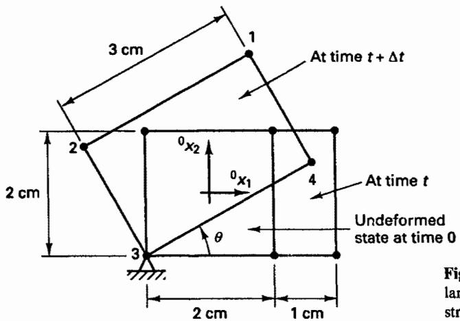EXAMPLE 6.13: A four-node element is stretched until time t and then undergoes without distortion a large rigid body rotation from time t to time $t + \Delta t$ as depicted in Fig. E6.13. Show explicitly that for the element the components of the Green-Lagrange strain tensor at time t and time $t + \Delta t$ are exactly equal. 

text_image

3 cm 1 At time t + Δt 2 0x2 0x1 4 At time t 3 θ 2 cm 1 cm Undeformed state at time 0 Fig lan str

Figure E6.13 Element subjected to large rigid body rotation after initial stretch The Green-Lagrange strain components at time t can be evaluated by inspection using (6.51), $$ _ {0} ^ {\prime} \epsilon_ {2 2} = 0; \quad_ {0} ^ {\prime} \epsilon_ {1 2} = _ {0} ^ {\prime} \epsilon_ {2 1} = 0 $$ and $\delta\epsilon_{11}=\frac{1}{2}\left[\left(\frac{3}{2}\right)^{2}-1\right]$ $=\frac{5}{8}$ Hence, $f_{0}\pmb{\epsilon} = \begin{bmatrix} \frac{5}{8} & 0\\ 0 & 0 \end{bmatrix}$ Alternatively, we can use (6.54), where we first evaluate the deformation gradient as in Example 6.6: $$ \mathbf {\delta} _ {0} ^ {t} \mathbf {X} = \left[ \begin{array}{l l} \frac {3}{2} & 0 \\ 0 & 1 \end{array} \right] $$ Hence, $\delta \mathbf{C} = \begin{bmatrix} \frac{9}{4} & 0 \\ 0 & 1 \end{bmatrix}$ and as before, $0^{\prime}\epsilon = \begin{bmatrix} \frac{5}{8} & 0 \\ 0 & 0 \end{bmatrix}$ (a) After the rigid body rotation the nodal point coordinates are

Node	$t+\Delta t_{x_1}$	$t+\Delta t_{x_2}$
1	$3\cos\theta-1-2\sin\theta$	$3\sin\theta-1+2\cos\theta$
2	$-1-2\sin\theta$	$2\cos\theta-1$
3	$-1$	$-1$
4	$3\cos\theta-1$	$3\sin\theta-1$

Thus, using again the procedure in Example 6.6 to evaluate the deformation gradient, we obtain $$ { } ^ { t + \Delta _ { 0 } ^ { t } } \mathbf { X } = \frac { 1 } { 4 } \left[ \begin{array} { c c } ( 1 + { } ^ { 0 } x _ { 2 } ) ( 3 \cos \theta - 1 - 2 \sin \theta ) & ( 1 + { } ^ { 0 } x _ { 1 } ) ( 3 \cos \theta - 1 - 2 \sin \theta ) \\ - ( 1 + { } ^ { 0 } x _ { 2 } ) ( - 1 - 2 \sin \theta ) & + ( 1 - { } ^ { 0 } x _ { 1 } ) ( - 1 - 2 \sin \theta ) \\ - ( 1 - { } ^ { 0 } x _ { 2 } ) ( - 1 ) & - ( 1 - { } ^ { 0 } x _ { 1 } ) ( - 1 ) \\ + ( 1 - { } ^ { 0 } x _ { 2 } ) ( 3 \cos \theta - 1 ) & - ( 1 + { } ^ { 0 } x _ { 1 } ) ( 3 \cos \theta - 1 ) \\ \hline ( 1 + { } ^ { 0 } x _ { 2 } ) ( 3 \sin \theta - 1 + 2 \cos \theta ) & ( 1 + { } ^ { 0 } x _ { 1 } ) ( 3 \sin \theta - 1 + 2 \cos \theta ) \\ - ( 1 + { } ^ { 0 } x _ { 2 } ) ( 2 \cos \theta - 1 ) & + ( 1 - { } ^ { 0 } x _ { 1 } ) ( 2 \cos \theta - 1 ) \\ - ( 1 - { } ^ { 0 } x _ { 2 } ) ( - 1 ) & - ( 1 - { } ^ { 0 } x _ { 1 } ) ( - 1 ) \\ + ( 1 - { } ^ { 0 } x _ { 2 } ) ( 3 \sin \theta - 1 ) & - ( 1 + { } ^ { 0 } x _ { 1 } ) ( 3 \sin \theta - 1 ) \end{array} \right] \tag {b} $$ or $t+\Delta t_{0}X=\begin{bmatrix}\frac{3}{2}\cos\theta&-\sin\theta\\ \frac{3}{2}\sin\theta&\cos\theta\end{bmatrix}$ (c) In reference to (6.29) we note that this deformation gradient can be written as $$ { } _ { 0 } ^ { t + \Delta t } \mathbf { X } = { } _ { t } ^ { t + \Delta t } \mathbf { R } \quad { } _ { 0 } ^ { t } \mathbf { U } \tag {d} $$ where $t+\Delta_{t}^{t}R=\begin{bmatrix}\cos\theta & -\sin\theta\\ \sin\theta & \cos\theta\end{bmatrix};\quad_{0}^{t}U=\begin{bmatrix}\frac{3}{2}&0\\ 0&1\end{bmatrix}$ This decomposition certainly corresponds to the actual physical situation, in which we measured a stretch in the $^0 x_1$ direction and then a rotation. Therefore, we could have established $^{t + \Delta t}X$ using (d) instead of performing all the calculations leading to (b) and thus (c)! Using (d) and (6.27), we obtain $$ { } _ { 0 } ^ { t + \Delta t } \mathbf { C } = \left[ \begin{array} { c c } \frac { 9 } { 4 } & 0 \\ 0 & 1 \end{array} \right] $$ and thus using (6.54), we have $$ { } ^ { t + \Delta t } _ { 0 } \epsilon = \left[ \begin{array} { c c } \frac { 5 } { 8 } & 0 \\ 0 & 0 \end{array} \right] \tag {e} $$ Hence $\delta \in$ in (a) is equal to $t + \frac{\Delta t}{0} \in$ in (e), which shows that the Green-Lagrange strain components did not change as a result of the rigid body rotation. EXAMPLE 6.14: Show that the components of the second Piola-Kirchhoff stress tensor are invariant under a rigid body rotation of the material. Here we consider a stationary coordinate system $x_{i}, i = 1, 2, 3$ and assume that the second Piola-Kirchhoff stress components are given in $\delta \mathbf{S}$ . Let the Cauchy stress, deformation gradient, and mass density at time $t$ be $\tau$ , $\delta \mathbf{X}$ , and $\rho$ . Hence, $$ _ {0} \mathbf {S} = \frac {{} ^ {0} \rho}{{} ^ {t} \rho} ^ {0} \mathbf {X} ^ {\prime} \boldsymbol {\tau} ^ {0} \mathbf {X} ^ {T} \tag {a} $$ where $^{0}$ X is the inverse deformation gradient. If a rigid body rotation is applied to the material from time t to time $t + \Delta t$ , the deformation gradient changes to $$ { } ^ { t + \Delta _ { 0 } ^ { t } } \mathbf { X } = \mathbf { R } { } _ { 0 } ^ { t } \mathbf { X } $$ where $\mathbf{R}$ is an orthogonal (rotation) matrix, and hence $$ { } _ { t + \Delta t } ^ { 0 } \mathbf { X } = { } _ { t } ^ { 0 } \mathbf { X } \mathbf { R } ^ { T } \tag {b} $$ Equations (a) and (b) show that $$ { } _ { 0 } ^ { t + \Delta t } \mathbf { S } = \frac { { } ^ { 0 } \rho } { { } ^ { t } \rho } { } _ { t } ^ { 0 } \mathbf { X } \mathbf { R } ^ { T } { } ^ { t + \Delta t } \mathbf { \tau } \mathbf { R } { } _ { t } ^ { 0 } \mathbf { X } ^ { T } \tag {c} $$ During the rigid body rotation of the material, the stress components remain constant in the rotating coordinate system. Hence the Cauchy stresses at time $t + \Delta t$ are in the fixed coordinate system, $$ { } ^ { t + \Delta t } \pmb { \tau } = \pmb { R } { } ^ { t } \pmb { \tau } \pmb { R } ^ { T } \tag {d} $$ Substituting from (d) into (c), we obtain $$ { } ^ { t + \Delta } { } _ { 0 } ^ { t } \mathbf { S } = \frac { { } ^ { 0 } \rho } { { } ^ { t } \rho } { } ^ { 0 } { } _ { t } \mathbf { X } ^ { T } { } ^ { t } { } _ { T } { } ^ { 0 } { } _ { t } \mathbf { X } ^ { T } $$ which completes the proof. Note that the reason for the second Piola-Kirchhoff stress components not to change is that the same matrix $\mathbf{R}$ is used in equations (b) and (d). 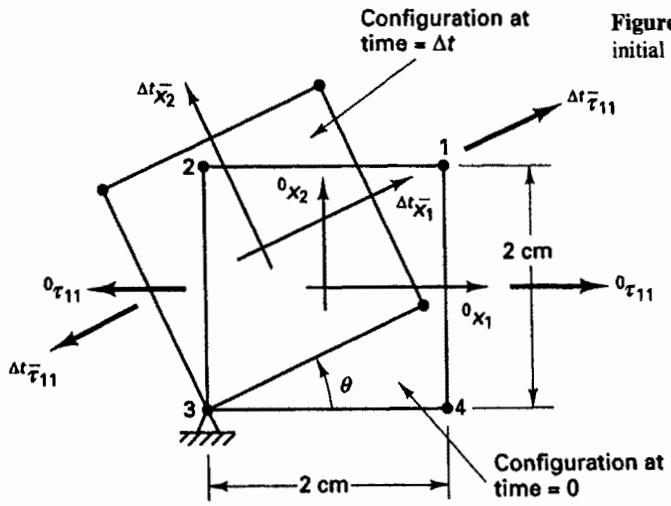EXAMPLE 6.15: Figure E6.15 shows a four-node element in the configuration at time 0. The element is subjected to a stress (initial stress) of $^{0}\tau_{11}$ . Assume that the element is rotated in time 0 to time $\Delta t$ as a rigid body through a large angle $\theta$ and that the stress in a body-attached coordinate system does not change. Hence, the magnitude of $\Delta t\bar{\tau}_{11}$ shown in Fig. E6.15 is equal to $^{0}\tau_{11}$ . Show that the components of the second Piola-Kirchhoff stress tensor did not change as a result of the rigid body rotation. 

text_image

Configuration at time = Δt Δt̅x̅₂ 0x₂ Δt̅x̅₁ 2 cm 0x₁ 0τ₁₁ Δt̅τ̅₁₁ θ 3 4 2 cm Configuration at time = 0 Figure initial

Figure E6.15 Four-node element with initial stress subjected to large rotation The second Piola-Kirchhoff stress tensor at time 0 is equal to the Cauchy stress tensor because the element deformations are zero, $$ \mathbf {S} = \left[ \begin{array}{l l} ^ 0 \tau_ {1 1} & 0 \\ 0 & 0 \end{array} \right] \tag {a} $$ The components of the Cauchy stress tensor at time $\Delta t$ expressed in the coordinate axes $^{0}x_{1}$ , $^{0}x_{2}$ are $$ \Delta t _ {\boldsymbol {\tau}} = \left[ \begin{array}{c c} \cos \theta & - \sin \theta \\ \sin \theta & \cos \theta \end{array} \right] \left[ \begin{array}{c c} \Delta t \overline {{\tau}} _ {1 1} & 0 \\ 0 & 0 \end{array} \right] \left[ \begin{array}{c c} \cos \theta & \sin \theta \\ - \sin \theta & \cos \theta \end{array} \right] \tag {b} $$ This transformation corresponds to a second-order tensor transformation of the components $\Delta^{t}\overline{\tau}_{ij}$ from the body-attached coordinate frame $\Delta^{t}\overline{x}_{1}$ , $\Delta^{t}\overline{x}_{2}$ to the stationary coordinate frame $^{0}x_{1}$ , $^{0}x_{2}$ (see Section 2.4). The relation between the Cauchy stresses and the second Piola-Kirchhoff stresses at time $\Delta t$ is, according to (6.68), $$ { } ^ { \Delta t } \mathbf { T } = \frac { { } ^ { \Delta t } \rho } { { } ^ { 0 } \rho } { } ^ { \Delta t } \mathbf { X } { } ^ { \Delta t } { } ^ { 0 } \mathbf { S } { } ^ { \Delta t } { } ^ { 0 } \mathbf { X } ^ { T } \tag {c} $$ where in this case $\Delta^t\rho /^0\rho = 1$ . The deformation gradient can be evaluated as in Example 6.6, where we note that the nodal point coordinates at time $t$ are $$ ^ {\Delta t} x _ {1} ^ {1} = 2 \cos \theta - 1 - 2 \sin \theta ; \quad^ {\Delta t} x _ {2} ^ {1} = 2 \sin \theta - 1 + 2 \cos \theta $$ $$ ^ {\Delta t} x _ {1} ^ {2} = - 1 - 2 \sin \theta ; \quad^ {\Delta t} x _ {2} ^ {2} = 2 \cos \theta - 1 $$ $$ ^ {\Delta t} x _ {1} ^ {3} = - 1; \quad^ {\Delta t} x _ {2} ^ {3} = - 1 $$ $$ ^ {\Delta t} x _ {1} ^ {4} = 2 \cos \theta - 1; \quad^ {\Delta t} x _ {2} ^ {4} = 2 \sin \theta - 1 $$ Hence, using the derivatives of the interpolation functions given in Example 6.6, we have $$ \Delta_ {0} ^ {t} \mathbf {X} = \frac {1}{4} \left[ \begin{array}{l l} (1 + ^ {0} x _ {2}) (2 \cos \theta - 1 - 2 \sin \theta) & (1 + ^ {0} x _ {1}) (2 \cos \theta - 1 - 2 \sin \theta) \\ - (1 + ^ {0} x _ {2}) (- 1 - 2 \sin \theta) & + (1 - ^ {0} x _ {1}) (- 1 - 2 \sin \theta) \\ - (1 - ^ {0} x _ {2}) (- 1) & - (1 - ^ {0} x _ {1}) (- 1) \\ + (1 - ^ {0} x _ {2}) (2 \cos \theta - 1) & - (1 + ^ {0} x _ {1}) (2 \cos \theta - 1) \\ \hline (1 + ^ {0} x _ {2}) (2 \sin \theta - 1 + 2 \cos \theta) & (1 + ^ {0} x _ {1}) (2 \sin \theta - 1 + 2 \cos \theta) \\ - (1 + ^ {0} x _ {2}) (2 \cos \theta - 1) & + (1 - ^ {0} x _ {1}) (2 \cos \theta - 1) \\ - (1 - ^ {0} x _ {2}) (- 1) & - (1 - ^ {0} x _ {1}) (- 1) \\ + (1 - ^ {0} x _ {2}) (2 \sin \theta - 1) & - (1 + ^ {0} x _ {1}) (2 \sin \theta - 1) \end{array} \right] $$ or $$ \Delta_ {0} ^ {t} \mathbf {X} = \left[ \begin{array}{c c} \cos \theta & - \sin \theta \\ \sin \theta & \cos \theta \end{array} \right] \tag {d} $$ Substituting now from (b) and (d) into (c), we obtain $$ \Delta_ {0} ^ {t} \mathbf {S} = \left[ \begin{array}{c c} \Delta^ {t} \overline {{\tau}} _ {1 1} & 0 \\ 0 & 0 \end{array} \right] \tag {e} $$ But, since $\Delta^{t}\overline{\tau}_{11}$ is equal to $^{0}\tau_{11}$ , the relations in (a) and (e) show that the components of the second Piola-Kirchhoff stress tensor did not change during the rigid body rotation. The reason there is no change in the second Piola-Kirchhoff stress tensor is that the deformation gradient corresponds in this case to the rotation matrix that is used in the transformation in (b). It is important to note that in these examples we consider the coordinate system to remain stationary and the body of material to be moving in this coordinate system. This situation is of course quite different from expressing given stress and strain tensors in new coordinate systems. The above relationships between the stresses and strains show that, using (6.69) for the stress transformation and (6.64) for the strain transformation (but, as in Example 6.10, using variations in strains rather than time derivatives), we obtain $$ \begin{array}{l} \int_ {t _ {V}} ^ {t} \tau_ {k l} \delta_ {t} e _ {k l} d ^ {t} V = \int_ {t _ {V}} \left(\frac {^ t \rho}{^ 0 \rho} _ {0} ^ {t} S _ {i j} ^ {t} _ {0} ^ {t} x _ {k, i} ^ {t} _ {0} ^ {t} x _ {l, j}\right) \left(_ {t} ^ {0} x _ {m, k} ^ {0} _ {t} x _ {n, l} \delta_ {0} ^ {t} \epsilon_ {m n}\right) d ^ {t} V \\ = \int_ {t _ {V}} \frac {^ {t} \rho}{^ {0} \rho} \delta S _ {i j} \delta_ {m i} \delta_ {n j} \delta_ {0} ^ {t} \epsilon_ {m n} d ^ {t} V = \int_ {0 _ {V}} \delta S _ {i j} \delta_ {0} ^ {t} \epsilon_ {i j} d ^ {0} V \tag {6.70} \\ \end{array} $$ where we have also used that $^{\prime}\rho d^{\prime}V = ^{0}\rho d^{0}V$ . Of course, (6.70) follows from the definition of the second Piola-Kirchhoff stress tensor in (6.66), and indeed (6.70) is but (6.66) in integrated form over the volume of the body (and written for strain variations). We have used in (6.70) a specific Cartesian coordinate system and should note that (6.70) is of course in component form a general tensor equation. Other suitable coordinate systems could also be chosen [see (6.178)]. Equation (6.70) is the basic expression of the total and updated Lagrangian formulations used in the incremental analysis of solids and structures, which we consider next. An important aspect of (6.70) is that in the final expression the integration is performed over the initial volume of the body. Instead of the initial configuration, any other previously calculated configuration could be used, with the second Piola-Kirchhoff stresses and Green-Lagrange strains then defined with respect to that configuration. More specifically, if the configuration at time $\tau$ is to be used, $\tau < t$ , and we denote the coordinates at that time by $\tau x_{i}$ , then we would employ $$ \int_ {t _ {V}} ^ {t} \tau_ {m n} \delta_ {t} e _ {m n} d ^ {t} V = \int_ {\tau_ {V}} ^ {t} S _ {i j} \delta_ {\tau} ^ {t} \epsilon_ {i j} d ^ {\tau} V \tag {6.71} $$ where the second Piola-Kirchhoff stresses $\tau S_{ij}$ and Green-Lagrange strains $\tau \epsilon_{ij}$ are defined as previously discussed, but instead of $^{0}x_{i}$ , the coordinates $^{7}x_{i}$ corresponding to the configuration at time $\tau$ are used. We shall employ the relations in (6.70) and (6.71) often in the next sections. Note that so far we have defined the stress and strain tensors that we shall employ; the use of appropriate constitutive relations is discussed in Section 6.6. # 6.2.3 Continuum Mechanics Incremental Total and Updated Lagrangian Formulations, Materially-Nonlinear-Only Analysis We discussed in Sections 6.1 and 6.2.1 the basic difficulties and the solution approach when a general nonlinear problem is analyzed, and we concluded that, for an effective incremental analysis, appropriate stress and strain measures need to be employed. This led in Section 6.2.2 to the presentation of some stress and strain tensors that are employed effectively in practice, and then to the principle of virtual displacements expressed in terms of second Piola-Kirchhoff stresses and Green-Lagrange strains. We now use this fundamental result in the development of two general continuum mechanics incremental formulations of nonlinear problems. We consider in this section only the continuum mechanics equations without reference to a particular finite element solution scheme. The use of the results and the generalization for incremental formulations with respect to general finite element solution variables are then discussed in Section 6.3.1 (and the sections thereafter). The basic equation that we want to solve is relation (6.13), which expresses the equilibrium and compatibility requirements of the general body considered in the configuration corresponding to time $t + \Delta t$ . [The constitutive equations also enter (6.13), namely, in the calculation of the stresses.] Since in general the body can undergo large displacements and large strains and the constitutive relations are nonlinear, the relation in (6.13) cannot be solved directly; however, an approximate solution can be obtained by referring all variables to a previously calculated known equilibrium configuration and linearizing the resulting equation. This solution can then be improved by iteration. To develop a governing linearized equation, we recall that the solutions for times 0, $\Delta t$ , $2\Delta t$ , $\ldots$ , t have already been calculated and that we can employ (6.70) or (6.71) and refer the stresses and strains to one of these known equilibrium configurations. Hence, in principle, any one of the equilibrium configurations already calculated could be used. In practice, however, the choice lies essentially between two formulations which have been termed total Lagrangian (TL) and updated Lagrangian (UL) formulations (see K. J. Bathe, E. Ramm, and E. L. Wilson [A]). The TL formulation has also been referred to as the Lagrangian formulation. In this solution scheme all static and kinematic variables are referred to the initial configuration at time 0. The UL formulation is based on the same procedures that are used in the TL formulation, but in the solution all static and kinematic variables are referred to the last calculated configuration. Both the TL and UL formulations include all kinematic nonlinear effects due to large displacements, large rotations, and large strains, but whether the large strain behavior is modeled appropriately depends on the constitutive relations specified (see Section 6.6). The only advantage of using one formulation rather than the other lies in its greater numerical efficiency. Using (6.70), in the TL formulation we consider the basic equation $$ \int_ {0 _ {V}} ^ {t + \Delta t} S _ {i j} \delta^ {t + \Delta t} \epsilon_ {i j} d ^ {0} V = ^ {t + \Delta t} \mathcal {R} \tag {6.72} $$ whereas in the UL formulation we consider $$ \int_ {t _ {V}} ^ {t + \Delta t} S _ {i j} \delta^ {t + \Delta t} \epsilon_ {i j} d ^ {t} V = ^ {t + \Delta t} \mathcal {R} \tag {6.73} $$ in which $^{t+\Delta t}\mathcal{R}$ is the external virtual work given in (6.14). This expression also depends in general on the surface area and the volume of the body under consideration. However, for simplicity of discussion we assume for the moment that the loading is deformation-independent, a very important form of such loading being concentrated forces whose directions and intensities are independent of the structural response. Later we shall discuss how to include deformation-dependent loading in the analysis [see (6.83) and (6.84)]. Tables 6.2 and 6.3 summarize the relations used to arrive at the linearized equations of motion about the state at time t in the TL and UL formulations. The linearized equilibrium equations are, in the TL formulation, $$ \int C _ {i j r s} e _ {r s} \delta_ {0} e _ {i j} d ^ {0} V + \int ^ {t} S _ {i j} \delta_ {0} \eta_ {i j} d ^ {0} V = ^ {t + \Delta t} \mathcal {R} - \int ^ {t} S _ {i j} \delta_ {0} e _ {i j} d ^ {0} V \tag {6.74} $$ and in the UL formulation $$ \int_ {t _ {V}} ^ {t} C _ {i j r s} ^ {t} e _ {r s} \delta_ {t} e _ {i j} d ^ {t} V + \int_ {t _ {V}} ^ {t} \tau_ {i j} \delta_ {t} \eta_ {i j} d ^ {t} V = ^ {t + \Delta t} \mathcal {R} - \int_ {t _ {V}} ^ {t} \tau_ {i j} \delta_ {t} e _ {i j} d ^ {t} V \tag {6.75} $$