```csv
COMMON/UNIM1/NPOIN, NELEM, NBOUN, NLOAD, NPROP, NNODE, IINCS, IITER, STF3 7
. KRESL, NCHEK, TOLER, NALGO, NSVAB, NDOFN, NINCS, NEVAB, STF3 8
. NITER, NOUTP, FACTO, PVALU STF3 9
COMMON/UNIM2/PROPS(5,4), COORD(26), LNODS(25,2), IFPRE(52), STF3 10
. FIXED(52), TLOAD(25,4), RLOAD(25,4), ELOAD(25,4), STF3 11
. MATNO(25), STRES(25,2), PLAST(25), XDISP(52), STF3 12
. TDISP(26,2), TREAC(26,2), ASTIF(52,52), ASLOD(52), STF3 13
. REACT(52), FRESV(1352), PEFIX(52), ESTIF(4,4) STF3 14
REWIND 1 STF3 15
DO 10 IELEM=1, NELEM STF3 16
LPROP=MATNO(IELEM) STF3 17
YOUNG=PROPS(LPROP,1) STF3 18
XAREA=PROPS(LPROP,2) STF3 19
HARDS=PROPS(LPROP,4) STF3 20
NODE1=LNODS(IELEM,1) STF3 21
NODE2=LNODS(IELEM,2) STF3 22
ELENG=ABS(COORD(NODE1)-COORD(NODE2)) STF3 23
FMULT=YOUNG*XAREA/ELENG STF3 24
IF(PLAST(IELEM).GT.0.0) FMULT=FMULT*(1.0-YOUNG/(YOUNG+HARDS)) STF3 25
ESTIF(1,1)=FMULT STF3 26
ESTIF(1,2)=-FMULT STF3 27
ESTIF(2,1)=-FMULT STF3 28
ESTIF(2,2)=FMULT STF3 29
WRITE(1) ESTIF STF3 30
10 CONTINUE STF3 31
RETURN STF3 32
END STF3 33
```
| STF3 15 | Rewind the file on which the stiffness matrix of each element will be stored. |
| STF3 16 | Loop over each element. |
| STF3 17 | Identify the material property of each element. |
| STF3 18 | Set YOUNG equal to the material elastic modulus. |
| STF3 19 | Set XAREA equal to the cross-sectional area. |
| STF3 20 | Set HARDS equal to the strain hardening parameter, $H'$ . |
| STF3 21–22 | Identify the node numbers of the element. |
| STF3 23 | Calculate the element length. |
| STF3 24 | Compute the multiplying term in (2.38) as FMULT. |
| STF3 25 | Check if the element has yielded. If yes, compute FMULT as the multiplying term in (2.43). |
| STF3 26–29 | Compute the components of the stiffness matrix. |
| STF3 30 | Write the element stiffness matrix on to disc file. |
| STF3 31 | Termination of DO LOOP over each element. |
# 3.12.2 Residual force subroutine, REFOR3
The purpose of this subroutine is to calculate the equivalent nodal forces from which the residual nodal forces will be evaluated in subroutine CONUND. In view of the essentially incremental nature of the equations of plasticity, the subroutine is somewhat more intricate than the residual force
subroutines developed to date. All stress and strain components must be accumulated from the values obtained during each iteration. The situation is further complicated by the fact that an element may yield when the residual forces are applied as loads for any iteration. The precise load at which yielding begins will generally lie somewhere between the total load corresponding to the previous iteration and the total load for the present cycle. Consequently the yield load must be determined and the plastic strain computed for only the post yield portion of the load. The general procedure adopted is to determine the stress in each element so that the yield criterion is satisfied. If the actual stress in any element is greater than this permissible value, then the additional part is removed but is included in the residual force vector to maintain equilibrium.
Consider the situation existing for the $r^{th}$ iteration of any particular load increment. The solution algorithm employed is presented below.
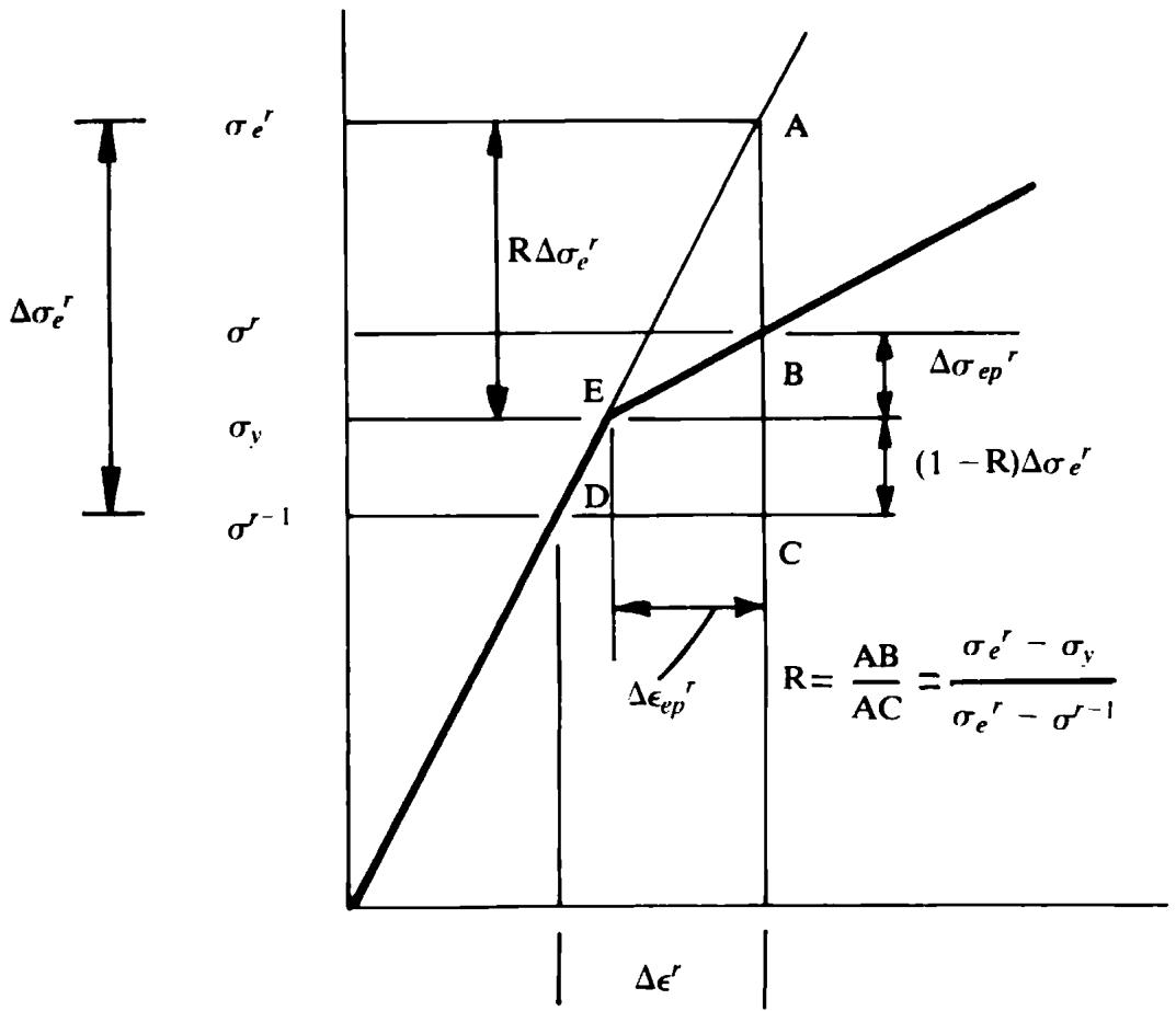
Step a The applied loads for the $r^{th}$ iteration are the residual forces $\psi^{r-1}$ calculated at the end of the $(r-1)^{th}$ iteration according to (2.4). These applied loads give rise to displacement increments, $\Delta\varphi^{r}$ , according to (2.12). Hence calculate the corresponding increment of strain $\Delta\epsilon^{r}$ . For the general element denote this value by $\Delta\epsilon^{r}$ and it is shown in Fig. 3.7.
Step b Compute the incremental stress change assuming linear elastic behaviour. This will introduce errors if the element has yielded and the material is behaving elasto-plastically. However, we will correct any discrepancy when the residual forces are calculated. Therefore we calculate the stress change according to $\Delta\sigma_{e}^{r}=E\Delta\epsilon^{r}$ , where the subscript e is used to denote that this stress is based on elastic behaviour.
Step c Accumulate the total stress for each element as $\sigma_{e}^{r} = \sigma^{r-1} + \Delta\sigma_{e}^{r}$ . The stress $\sigma^{r-1}$ will have been determined to satisfy the yield condition during the $(r-1)^{\text{th}}$ iteration. Consequently, the error in the stress $\sigma_{e}^{r}$ is limited to $\Delta\sigma_{e}^{r}$ . Again the subscript e denotes that $\sigma_{e}^{r}$ is based on an elastic behaviour.
Step d The next step in the process depends on whether or not the element had previously yielded on the $(r-1)^{\text{th}}$ iteration. This can be checked from the known value of the yield stress for the $(r-1)^{\text{th}}$ iteration. The stress limit for this cycle is given from Fig. 2.9 as
$$
\sigma_ {Y} ^ {r - 1} = \sigma_ {Y} + H ^ {\prime} \epsilon_ {p} ^ {r - 1}.
$$
Since the plastic strain $\epsilon_{p}$ will differ from element to element, each element will generally have a different permissible stress level.

text_image
σe^r
Δσe^r
σ^r
σy
σr^-1
RΔσe^r
A
E
B
Δσep^r
(1 - R)Δσe^r
D
C
Δεep^r
R = AB/AC = σe^r - σy/σe^r - σr^-1
Δε^r
(a)

line
| x-axis label | y-axis label | Description |
| ------------ | ------------ | ------------------- |
| Start | σₑʳ | |
| End | σʳ | Slope = E, Δσₑₚʳ, Δσₑₚʳ, r = 1 |
| End | σʳ | |
| End | σʳ⁻¹ | |
(b)
Fig. 3.7 Incremental stress and strain changes in a one-dimensional elasto-plastic material. (a) Initial yielding of material. (b) Material previously yielded.
Therefore we check if $\sigma^{r-1} > \sigma_Y + H' \epsilon_p^{r-1}$ . If the answer is:
# YES
which implies that the element had already yielded during the previous iteration, then check to see if $\sigma_{e}^{r} > \sigma^{r-1}$ . If the answer is:
NO
YES
The element is unloading which according to plasticity theory must take place elastically, and no further action need be taken. Go directly to Step g.
The element had reached the threshold stress during the previous iteration and the stress is still increasing. Therefore all the excess stress $\sigma_{e}^{r}-\sigma^{r-i}$ must be reduced to the yield value as indicated in Fig. 3.7(b). Therefore the factor, R, which defines the portion of the stress which must be modified to satisfy the yield condition, is equal to 1 in this case as shown in Fig. 3.7(b).
# NO
which implies that the element had not previously yielded. We now check to see if $\sigma_{e}^{r} > \sigma_{Y}$ . If the answer is:
NO
YES
The element is still elastic and no further action need be taken. Go directly to Step g.
The element has yielded during the application of load corresponding to this iteration as illustrated in Fig. 3.7(a). Therefore the portion of the stress greater than the yield value must be reduced to the elastoplastic line. The removed portion will be included in the residual force vector. The reduction factor, R, is found, with reference to Fig. 3.7(a) to be
$$
\begin{array}{l} R = \frac {A B}{A C} \\ = \frac {\sigma_ {e} ^ {r} - \sigma_ {Y}}{\sigma_ {e} ^ {r} - \sigma^ {r - 1}}. \\ \end{array}
$$
Step e For yielded elements only, calculate the increment of stress $\Delta\sigma_{ep}^{k}$ , which is the portion after yielding, permitted by elasto-plastic theory. This stress value is shown in Fig. 3.7 for the two cases when (a) yielding has commenced during this iteration and (b) when the element had previously yielded. Using (2.4) we have
$$
\Delta \sigma_ {e p} ^ {r} = E \left(1 - \frac {E}{E + H ^ {\prime}}\right) \Delta \epsilon_ {e p} ^ {r}, \tag {3.33}
$$
where the subscript $ep$ denotes elasto-plastic behaviour. For the above to be generally true we must restrict ourselves to small increments of stress and strain. For the situation of Fig. 3.7(a), noting that triangles ADC and AEB are similar, we have
$$
\Delta \epsilon_ {e p} ^ {r} = R \Delta \epsilon^ {r}. \tag {3.34}
$$
Defining R = 1 for the situation of Fig. 3.7(b), then (3.34) is still correct. Therefore
$$
\Delta \sigma_ {e p} ^ {r} = E \left(1 - \frac {E}{E + H ^ {\prime}}\right) R \Delta \epsilon^ {r}. \tag {3.35}
$$
The total current stress is given by
$$
\sigma^ {r} = \sigma^ {r - 1} + (1 - R) \Delta \sigma_ {e} ^ {r} + \Delta \sigma_ {e p} ^ {r}, \tag {3.36}
$$
where the second term accounts for the elastic portion of the stress increment occurring before the onset of yielding.
Step f For yielded elements only, evaluate the total plastic strain for the element as $\epsilon_{p}^{r} = \epsilon_{p}^{r-1} + \Delta\epsilon_{p}^{r}$ where the plastic strain increment for the iteration is calculated as follows. For the elastic component of strain, $\Delta\epsilon_{e}^{r}$ , we have
$$
\Delta \epsilon_ {e} ^ {r} = \frac {\Delta \sigma^ {r}}{E}. \tag {3.37}
$$
Substituting for $\Delta\sigma^{r}$ from the linearised form of (2.35) into (3.37) and then using (2.34) we obtain
$$
\Delta \epsilon_ {p} ^ {r} = \frac {\Delta \epsilon^ {r}}{1 + H ^ {\prime} / E}. \tag {3.38}
$$
Since the plastic strain component must be calculated for the part of the strain after the element yields, then, with reference to Fig. 3.7, $\Delta\epsilon^{r}$ must be replaced by $\Delta\epsilon_{ep}^{r}$ . Or, using (3.34), we have
$$
\Delta \epsilon_ {p} ^ {r} = \frac {R \Delta \epsilon^ {r}}{1 + H ^ {\prime} / E}. \tag {3.39}
$$
Then the total current plastic strain for the element is
$$
\epsilon_ {p} ^ {r} = \epsilon_ {p} ^ {r - 1} + \frac {R \Delta \epsilon^ {r}}{1 + H ^ {\prime} / E}. \tag {3.40}
$$
Step g For elastic elements only, store the correct current stress as
$$
\sigma^ {r} = \sigma^ {r - 1} + \Delta \sigma_ {e} ^ {r}. \tag {3.41}
$$
(This in fact repeats Step c.)
Step h Finally, calculate the equivalent nodal forces from the element stress according to
$$
f _ {1} = - f _ {2} = \left\{ \begin{array}{c c c} - \sigma^ {r} A & \text {for} & x _ {2} > x _ {1} \\ \sigma^ {r} A & \text {for} & x _ {2} < x _ {1}. \end{array} \right. \tag {3.42}
$$
Subroutine REFOR3 is now presented below and explanatory notes provided.
```fortran
SUBROUTINE REFOR3 RFR3 1
C**************************RFR3 2
C RFR3 3
C *** CALCULATES INTERNAL EQUIVALENT NODAL FORCES RFR3 4
C RFR3 5
C**************************RFR3 6
COMMON/UNIM1/NPOIN,NELEM,NBOUN,NLOAD,NPROP,NNODE,IINCS,IITER, RFR3 7
. KRESL,NCHEK,TOLER,NALGO,NSVAB,NDOFN,NINCS,NEVAB, RFR3 8
. NITER,NOUTP,FACTO,PVALU RFR3 9
COMMON/UNIM2/PROPS(5,4),COORD(26),LNODS(25,2),IFPRE(52), RFR3 10
. FIXED(52),TLOAD(25,4),RLOAD(25,4),ELOAD(25,4), RFR3 11
. MATNO(25),STRES(25,2),PLAST(25),XDISP(52), RFR3 12
. TDISP(26,2),TREAC(26,2),ASTIF(52,52),ASLOD(52), RFR3 13
. REACT(52),FRESV(1352),PEFIX(52),ESTIF(4,4) RFR3 14
DO 10 IELEM=1,NELEM RFR3 15
DO 10 IEVAB=1,NEVAB RFR3 16
10 ELOAD(IELEM,IEVAB)=0.0 RFR3 17
DO 70 IELEM=1,NELEM RFR3 18
LPROP=MATNO(IELEM) RFR3 19
YOUNG=PROPS(LPROP,1) RFR3 20
XAREA=PROPS(LPROP,2) RFR3 21
YIELD=PROPS(LPROP,3) RFR3 22
HARDS=PROPS(LPROP,4) RFR3 23
NODE1=LNODS(IELEM,1) RFR3 24
NODE2=LNODS(IELEM,2) RFR3 25
ELENG=ABS(COORD(NODE1)-COORD(NODE2)) RFR3 26
IF(COORD(NODE2).GT.COORD(NODE1)) STRAN=(XDISP(NODE2)-XDISP(NODE1)) RFR3 27
./ELENG RFR3 28
IF(COORD(NODE2).LT.COORD(NODE1)) STRAN=(XDISP(NODE1)-XDISP(NODE2)) RFR3 29
./ELENG RFR3 30
STLIN=YOUNG*STRAN RFR3 31
STCUR=STRES(IELEM,1)+STLIN RFR3 32
PREYS=YIELD+HARDS*ABS(PLAST(IELEM)) RFR3 33
IF(ABS(STRES(IELEM,1)).GE.PREYS) GO TO 20 RFR3 34
ESCUR=ABS(STCUR)-PREYS RFR3 35
IF(ESCUR.LE.0.0) GO TO 40 RFR3 36
RFACT=ESCUR/ABS(STLIN) RFR3 37
GO TO 30 RFR3 38
20 IF(STRES(IELEM,1).GT.0.0.AND.STLIN.LE.0.0) GO TO 40 RFR3 39
IF(STRES(IELEM,1).LT.0.0.AND.STLIN.GT.0.0) GO TO 40 RFR3 40
RFACT=1.0 RFR3 41
30 REDUC=1.0-RFACT RFR3 42
STRES(IELEM,1)=STRES(IELEM,1)+REDUC*STLIN+RFACT*YOUNG*(1.0-
. YOUNG/(YOUNG+HARDS))*STRAN RFR3 44
PLAST(IELEM)=PLAST(IELEM)+RFACT*STRAN*YOUNG/(YOUNG+HARDS) RFR3 45
GO TO 50 RFR3 46
40 STRES(IELEM,1)=STRES(IELEM,1)+STLIN RFR3 47
50 IF(COORD(NODE2).GT.COORD(NODE1)) GO TO 60 RFR3 48
ELOAD(IELEM,1)=STRES(IELEM,1)*XAREA RFR3 49
ELOAD(IELEM,2)=-STRES(IELEM,1)*XAREA RFR3 50
GO TO 70 RFR3 51
60 ELOAD(IELEM,1)=-STRES(IELEM,1)*XAREA RFR3 52
ELOAD(IELEM,2)=STRES(IELEM,1)*XAREA RFR3 53
70 CONTINUE RFR3 54
RETURN RFR3 55
END RFR3 56
```
RFR3 15-17 Initialise to zero the array in which the equivalent nodal forces for each element will be stored.
RFR3 18 Loop over each element.
RFR3 19 Identify the material property of each element.
RFR3 20 Set YOUNG equal to the elastic modulus, E, of the material.
RFR3 21 Set XAREA equal to the cross-sectional area.
RFR3 22 Set YIELD equal to the uniaxial yield stress, $\sigma_{Y}$ , of the material.
RFR3 23 Set HARDS equal to the hardening parameter, $H'$ , of the material.
RFR3 24-25 Identify the node numbers of the element.
RFR3 26 Calculate the element length.
RFR3 27–30 Calculate the element strain, so that a tensile strain is positive.
RFR3 31 Calculate $\Delta \sigma_{e}^{r}$ according to Step b.
RFR3 32 Calculate $\sigma_{e}^{r}$ according to Step c.
RFR3 33–34 Check if the element had yielded on the previous iteration, i.e., if $\sigma^{r-1} > \sigma_{Y} + H' \epsilon_{p}^{r-1}$ which is the first operation of Step d. The absolute value of $\sigma^{r-1}$ is taken to account for yielding in compression.
RFR3 35–36 If the element was previously elastic, check to see if it has yielded during this iteration.
RFR3 37 For an element which yields during this iteration, calculate
$$
R = \frac {\sigma_ {e} ^ {r} - \sigma_ {Y}}{\sigma_ {e} ^ {r} - \sigma^ {r - 1}}
$$
(Fig. 3.7(a)). The absolute value sign is taken to account for compressive loading.
RFR3 39–40 Check to see if an element which had previously yielded is unloading during this iteration. If yes, go to 40.
RFR3 41 Otherwise, set R = 1.
RFR3 42 Evaluate, $(1 - R)$ .
RFR3 43–44 For plastic elements, calculate the correct current stress, $\sigma^{r}$ , according to (3.36).
RFR3 45 Also calculate the plastic strain, $\epsilon_{p}^{r}$ , according to (3.40).
RFR3 47 For elastic elements, calculate the current stress, $\sigma^{r}$ , according to Step g.
RFR3 48–53 Evaluate the equivalent nodal forces, according to Step h.
RFR3 54 Termination of DO LOOP over the elements.
# 3.12.3 Numerical examples
The first example considered is the yielding of a bar under self weight loading. The problem and finite element idealisation employed is illustrated in Fig. 3.8. Progressive yielding is induced in the system by increasing the gravitational field incrementally. The gravitational force due to self weight

line
| End displacement (node 6) | Reaction (node 1) |
| ------------------------- | ----------------- |
| 0.000 | 0.0 |
| 0.002 | 10.0 |
| 0.004 | 12.0 |
| 0.006 | 14.0 |
| 0.008 | 16.0 |
| 0.010 | 18.0 |
| 0.012 | 20.0 |
| 0.014 | 22.0 |
| 0.016 | 24.0 |
| 0.018 | 26.0 |
| 0.020 | 28.0 |
| 0.022 | 30.0 |
Fig. 3.8 Load/displacement response of a vertical bar loaded by a progressively increasing self-weight.
acting on each element is equally distributed to its two nodes. The structure is capable of carrying load beyond first yield, due to the strain hardening characteristic of the material.
The second example considered is the compound bar shown in Fig. 3.9. The two bars have a different yield stress and cross-sectional area in order to induce differential yielding. The structure is loaded by an end load, P, which is systematically incremented. The load/extension characteristics for the system are shown in Fig. 3.9. It is seen that there is an initial loss of stiffness corresponding to yielding of the first bar followed by a further reduction when the second bar becomes plastic.
This simple example suggests a method by which more complex material responses can be generated. By connecting two bars with different properties in parallel we obtain a material behaviour made up of three linear portions.

By connecting n bars in parallel and choosing the yield stress and cross-sectional area of each appropriately we can approximate any arbitrary stress/strain response piecewise linearly by $(n+1)$ intervals. This is the basis of the ‘overlay method’ $^{(7)}$ which will be described later in Chapter 8.
Also included in Fig. 3.9 are the results for the case when the load is cycled. First the load is incremented in tension up to a certain level, then removed and applied compressively, before final removal. It is immediately seen that a Bauschinger effect $^{(8)}$ is obtained with initial yield in compression taking place at a reduced value. This occurs even though we have assumed an equal yield stress in tension and compression. This behaviour is attributable to the differential straining of the two components and is a phenomenon evident in real materials.
# 3.13 Problems
3.1 Reanalyse the problem of Fig. 3.3, Section 3.9.3, for the case where the term K is assumed to vary with the unknown $\phi$ according to
$$
K = 1 0 (1 + e ^ {3 \phi}).
$$
Use the direct iteration solution code QUITER, user instructions for which are provided in Appendix I, Section A1.1, for solution.
3.2 Resolve Problem 3.1 using the Newton-Raphson procedure which is coded in program QUNEWT. User instructions for this program are provided in Appendix I, Section A1.2. Compare the computation times required for the two different solution procedures.
3.3 The quasi-harmonic equation described in Section 2.3 is also applicable to groundwater flow problems. $^{(5)}$ In this application $\phi$ is the pressure head potential, K is the material permeability and Q is the rate at which water is being injected per unit volume of material. The flow velocity at any point is then given by $v = -K(d\phi/dx)$ . Figure 3.10 illustrates the problem of water seeping through two permeable strata whose permeabilities depend on the seepage velocity as shown. By treating the problem as one-dimensional in the vertical direction obtain a numerical solution for the steady state potential and velocity distribution in the two strata.
3.4 Following the approach of Section 2.3, develop the stiffness matrix $H^{(e)}$ and the load vector $f^{(e)}$ for the one-dimensional axisymmetric situation. In this application all quantities are symmetric with respect to a central axis and the radial coordinate r now replaces x.
3.5 Implement the formulation of Problem 3.4 in program QUITER.
3.6 Use the computer code developed in Problem 3.5 to solve the problem of water flow in the horizontal place of the confined aquifer shown in Fig. 3.11. In this case $\phi$ is the piezometric head, K is the material permeability and Q is the rate at which water is being injected per unit volume of material.