| SUBROUTINE FLOWPL(AVECT,ABETA,DVECT,NTYPE,PROPS,LPROP,NSTR1,MMATS)FLPL | 1 |
| C*************** | FLPL 2 |
| C | FLPL 3 |
| C**** THIS SUBROUTINE EVALUATES THE PLASTIC D VECTOR | FLPL 4 |
| C | FLPL 5 |
| C*************** | FLPL 6 |
| DIMENSION AVECT(4),DVECT(4),PROPS(MMATS,7) | FLPL 7 |
| YOUNG=PROPS(LPROP,1) | FLPL 8 |
| POISS=PROPS(LPROP,2) | FLPL 9 |
| HARDS=PROPS(LPROP,6) | FLPL 10 |
| FMUL1=YOUNG/(1.0+POISS) | FLPL 11 |
| IF(NTYPE.EQ.1) GO TO 60 | FLPL 12 |
| FMUL2=YOUNG*POISS*(AVECT(1)+AVECT(2)+AVECT(4))/(1.0+POISS)* | FLPL 13 |
| .(1.0-2.0*POISS)) | FLPL 14 |
| DVECT(1)=FMUL1*AVECT(1)+FMUL2 | FLPL 15 |
| DVECT(2)=FMUL1*AVECT(2)+FMUL2 | FLPL 16 |
| DVECT(3)=0.5*AVECT(3)*YOUNG/(1.0+POISS) | FLPL 17 |
| DVECT(4)=FMUL1*AVECT(4)+FMUL2 | FLPL 18 |
| GO TO 70 | FLPL 19 |
| SUBROUTINE STIFFP(COORD,EPSTN,IINCS,LNODS,MATNO,MEVAB,MMATS, | STFP | 1 |
| . MPOIN,MTOTV,NELEM,NEVAB,NGAUS,NNODE,NSTRE, | STFP | 2 |
| . NSTR1,POSGP,PROPS,WEIGP,MELEM,MTOTG, | STFP | 3 |
| . STRSG,NTYPE,NCRIT) | STFP | 4 |
| C********** | STFP | 5 |
| C | STFP | 6 |
| C**** THIS SUBROUTINE EVALUATES THE STIFFNESS MATRIX FOR EACH ELEMENT | STFP | 7 |
| C IN TURN | STFP | 8 |
| C | STFP | 9 |
| C********** | STFP | 10 |
| DIMENSION BMATX(4,18),CARTD(2,9),COORD(MPOIN,2),DBMAT(4,18), | STFP | 11 |
| . DERIV(2,9),DEVIA(4),DMATX(4,4), | STFP | 12 |
| . ELCOD(2,9),EPSTN(MTOTG),ESTIF(18,18),LNODS(MELEM,9), | STFP | 13 |
| . MATNO(MELEM),POSGP(4),PROPS(MMATS,7),SHAPE(9), | STFP | 14 |
| . WEIGP(4),STRES(4),STRSG(4,MTOTG), | STFP | 15 |
| . DVECT(4),AVECT(4),GPCOD(2,9) | STFP | 16 |
| TWOPI=6.283185308 | STFP | 17 |
| REWIND 1 | STFP | 18 |
```csv
KGAUS=0
STFP 19
C
C*** LOOP OVER EACH ELEMENT
STFP 20
C
DO 70 IELEM=1,NELEM
STFP 21
LPROP=MATNO(IELEM)
STFP 22
STFP 23
STFP 24
C
C*** EVALUATE THE COORDINATES OF THE ELEMENT NODAL POINTS
STFP 25
C
DO 10 INODE=1,NNODE
STFP 26
LNODE=IABS(LNODS(IELEM,INODE))
STFP 27
IPOSN=(LNODE-1)*2
STFP 28
DO 10 IDIME=1,2
STFP 29
IPOSN=IPOSN+1
STFP 30
STFP 31
STFP 32
10 ELCOD(IDIME,INODE)=COORD(LNODE,IDIME)
STFP 33
THICK=PROPS(LPROP,3)
STFP 34
C
C*** INITIALIZE THE ELEMENT STIFFNESS MATRIX
STFP 35
C
DO 20 IEVAB=1,NEVAB
STFP 36
DO 20 JEVAB=1,NEVAB
STFP 37
20 ESTIF(IEVAB,JEVAB)=0.0
STFP 38
KGASP=0
STFP 39
KGASP=0
STFP 40
STFP 41
C
C*** ENTER LOOPS FOR AREA NUMERICAL INTEGRATION
STFP 42
C
DO 50 IGAUS=1,NGAUS
STFP 43
EXISP=POSGP(IGAUS)
STFP 44
DO 50 JGAUS=1,NGAUS
STFP 45
ETASP=POSGP(JGAUS)
STFP 46
KGASP=KGASP+1
STFP 47
KGASP=KGASP+1
STFP 48
STFP 49
STFP 50
C
C*** EVALUATE THE D-MATRIX
STFP 51
C
CALL MODPS(DMATX,LPROP,MMATS,NTYPE,PROPS)
STFP 52
C
C*** EVALUATE THE SHAPE FUNCTIONS,ELEMENTAL VOLUME,ETC.
STFP 53
C
CALL SFR2(DERIV,ETASP,EXISP,NNODE,SHAPE)
STFP 54
CALL JACOB2(CARTD,DERIV,DJACB,ELCOD,GPCOD,IELEM,KGASP,
NNODE,SHAPE)
STFP 55
DVOLU=DJACB*WEIGP(IGAUS)*WEIGP(JGAUS)
STFP 56
IF(NTYPE.EQ.3) DVOLU=DVOLU*TWOPI*GPCOD(1,KGASP)
STFP 57
IF(THICK.NE.0.0) DVOLU=DVOLU*THICK
STFP 58
C
C*** EVALUATE THE B AND DB MATRICES
STFP 59
STFP 60
STFP 61
STFP 62
STFP 63
C
C*** EVALUATE THE B AND DB MATRICES
STFP 64
C
CALL BMATPS(BMATX,CARTD,NNODE,SHAPE,GPCOD,NTYPE,KGASP)
STFP 65
IF(IINCS.EQ.1) GO TO 80
STFP 66
IF(EPSTN(KGAUS),EQ.0.0) GO TO 80
STFP 67
DO 90 ISTR1=1,NSTR1
STFP 68
STFP 69
STFP 70
90 STRES(ISTR1)=STRSG(ISTR1,KGAUS)
STFP 71
CALL INVAR(DEVIA,LPROP,MMATS,NCRIT,PROPS,SINT3,STEFF,STRES,
THETA,VARJ2,YIELD)
STFP 72
CALL YIELDF(AVECT,DEVIA,LPROP,MMATS,NCRIT,NSTR1,
PROPS,SINT3,STEFF,THETA,VARJ2)
STFP 73
CALL FLOWPL(AVECT,ABETA,DVECT,NTYPE,PROPS,LPROP,NSTR1,MMATS)
STFP 74
DO 100 ISTRE=1,NSTRE
STFP 75
DO 100 JSTRE=1,NSTRE
STFP 76
STFP 77
100 DMATX(ISTRE,JSTRE)=DMATX(ISTRE,JSTRE)-ABETA*DVECT(ISTRE)
STFP 78
DVECT(JSTRE)
STFP 79
STFP 80
80 CONTINUE
STFP 81
CALL DBE(BMATX,DBMAT,DMATX,MEVAB,NEVAB,NSTRE,NSTR1)
STFP 82
```
| C | STFP | 83 |
| C*** CALCULATE THE ELEMENT STIFFNESSES | STFP | 84 |
| C | STFP | 85 |
| DO 30 IEVAB=1,NEVAB | STFP | 86 |
| DO 30 JEVAB=IEVAB,NEVAB | STFP | 87 |
| DO 30 ISTRE=1,NSTRE | STFP | 88 |
| 30 ESTIF(IEVAB,JEVAB)=ESTIF(IEVAB,JEVAB)+BMATX(ISTRE,IEVAB)* | STFP | 89 |
| . DBMAT(ISTRE,JEVAB)*DVOLU | STFP | 90 |
| 50 CONTINUE | STFP | 91 |
| C | STFP | 92 |
| C*** CONSTRUCT THE LOWER TRIANGLE OF THE STIFFNESS MATRIX | STFP | 93 |
| C | STFP | 94 |
| DO 60 IEVAB=1,NEVAB | STFP | 95 |
| DO 60 JEVAB=1,NEVAB | STFP | 96 |
| 60 ESTIF(JEVAB,IEVAB)=ESTIF(IEVAB,JEVAB) | STFP | 97 |
| C | STFP | 98 |
| C*** STORE THE STIFFNESS MATRIX,STRESS MATRIX AND SAMPLING POINT | STFP | 99 |
| C COORDINATES FOR EACH ELEMENT ON DISC FILE | STFP | 100 |
| C | STFP | 101 |
| WRITE(1) ESTIF | STFP | 102 |
| 70 CONTINUE | STFP | 103 |
| RETURN | STFP | 104 |
| END | STFP | 105 |
STFP 17 Compute the value of $2\pi$ .
STFP 18 Rewind the disc file on which the element stiffness matrices will be stored in turn.
STFP 19 Set to zero the counter which indicates the overall Gauss point location. So KGAUS ranges from 1 to NGAUS\*NGAUS\*NELEM.
STFP 23 Enter the loop over each element in the structure.
STFP 24 Identify the material property type of the current element.
STFP 28-33 Store the element nodal coordinates in the local array ELCOD for convenient use later.
STFP 34 Identify the element thickness.
STFP 38–40 Zero the element stiffness array.
STFP 41 Set to zero the element Gauss point counter. So KGASP ranges from 1 to NGAUS\*NGAUS.
STFP 45–48 Enter the numerical integration loops and locate the position $(\xi, \eta)$ of the current point.
STFP 49–50 Increment the local and global Gauss point counters.
STFP 54 Call subroutine MODPS to evaluate the elasticity matrix, D.
STFP 58 Evaluate the shape functions $N_{i}$ and the derivatives $\partial N_{i}/\partial\xi$ , $\partial N_{i}/\partial\eta$ for the current Gauss point.
STFP 59–60 Evaluate the Gauss point coordinates, GPCOD(IDIME, KGASP), the determinant of the Jacobian matrix, $|J|$ and the Cartesian derivatives of the shape functions $\partial N_{i}/\partial x$ , $\partial N_{i}/\partial y$ (or $\partial N_{i}/\partial r$ , $\partial N_{i}/\partial z$ for axisymmetric problems).
STFP 61–63 Calculate the elemental volume for numerical integration as $|J|W_{\xi}W_{\eta}$ taking care to multiply by the appropriate thickness or by $2\pi r$ for axisymmetric problems. Note that if a zero thickness is specified it is automatically taken to be unity.
STFP 67 Evaluate the B matrix.
STFP 68 For the first time avoid the replacement of D by $D_{ep}$ , as defined in (7.47).
STFP 69 Also for Gauss points at which the behaviour is elastic avoid the replacement of D by $D_{ep}$ .
STFP 70-71 Store the total current stresses in the array STRES.
STFP 72-76 Call subroutines INVAR, YIELDF and FLOWPL to evaluate the vectors $a$ , (AVECT) and $d_{D}$ , (DVECT) and ABETA = $1/(H' + d_{D}^{T}a)$ .
STFP 77-80 Evaluate $D_{ep}$ according to (7.47).
STFP 82 Evaluate $D_{ep}B$ .
STFP 86-90 Compute the upper triangle of the element stiffness matrix as
$$
\int_ {\Omega} \boldsymbol {B} ^ {T} \boldsymbol {D} _ {e p} \boldsymbol {B} d \Omega
$$
STFP 91 End of loop for numerical integration.
STFP 95–97 Complete the lower triangle of the element stiffness matrix by symmetry.
STFP 102 Store the element stiffness matrix on disc file 1.
STFP 103 Return to process the next element.
# 7.8.6 Subroutine LINEAR
The purpose of this subroutine is merely to determine the stresses from given displacements assuming linear elastic behaviour. This subroutine is employed in the residual force calculation to be described in the next section. The element displacement components, ELDIS(IDOFN, INODE) are entered into the subroutine, the strain components at the Gauss point under consideration, STRAN(ISTR1) calculated and finally the stress components are evaluated and stored in STRES(ISTR1).
The subroutine is now listed and described.
```csv
SUBROUTINE LINEAR(CARTD,DMATX,ELDIS,LPROP,MMATS,NDOFN,NNODE,NSTRE,LINR 1
NTYPE,PROPS,STRAN,STRES,KGASP,GPCOD,SHAPE) LINR 2
C********** LINR 3
C LINR 4
C**** THIS SUBROUTINE EVALUATES STRESSES AND STRAINS ASSUMING LINEAR LINR 5
C ELASTIC BEHAVIOUR LINR 6
C LINR 7
C********** LINR 8
DIMENSION AGASH(2,2),CARTD(2,9),DMATX(4,4),ELDIS(2,9), LINR 9
PROPS(MMATS,7),STRAN(4),STRES(4), LINR 10
GPCOD(2,9),SHAPE(9) LINR 11
POISS=PROPS(LPROP,2) LINR 12
DO 20 IDOFN=1,NDOFN LINR 13
DO 20 JDOFN=1,NDOFN LINR 14
BGASH=0.0 LINR 15
DO 10 INODE=1,NNODE LINR 16
```
10 BGASH=BGASH+CARTD(JDOFN,INODE)*ELDIS(IDOFN,INODE) LINR 17
20 AGASH(IDOFN,JDOFN)=BGASH LINR 18
C LINR 19
C*** CALCULATE THE STRAINS LINR 20
C LINR 21
STRAN(1)=AGASH(1,1) LINR 22
STRAN(2)=AGASH(2,2) LINR 23
STRAN(3)=AGASH(1,2)+AGASH(2,1) LINR 24
STRAN(4)=0.0 LINR 25
DO 30 INODE=1,NNODE LINR 26
30 STRAN(4)=STRAN(4)+ELDIS(1,INODE)*SHAPE(INODE)/GPCOD(1,KGASP) LINR 27
C LINR 28
C*** AND THE CORRESPONDING STRESSES LINR 29
C LINR 30
DO 40 ISTRE=1,NSTRE LINR 31
STRES(ISTRE)=0.0 LINR 32
DO 40 JSTRE=1,NSTRE LINR 33
40 STRES(ISTRE)=STRES(ISTRE)+DMATX(ISTRE,JSTRE)*STRAN(JSTRE) LINR 34
IF(NTYPE.EQ.1) STRES(4)=0.0 LINR 35
IF(NTYPE.EQ.2) STRES(4)=POISS*(STRES(1)+STRES(2)) LINR 36
RETURN LINR 37
END LINR 38
LINR 12 Identify POISS as the Poisson's ratio of the element material.
LINR 13-18 Calculate the Cartesian derivatives of the Gauss point displacement components $\partial u / \partial x$ , $\partial u / \partial y$ , $\partial v / \partial x$ , $\partial v / \partial y$ .
LINR 22-27 Evaluate the strain components at the Gauss point according to
$$
\epsilon = \left\{ \begin{array}{l} \epsilon_ {x} \\ \epsilon_ {y} \\ \gamma_ {x y} \\ \epsilon_ {z}. \end{array} \right\} = \left\{ \begin{array}{c} \frac {\partial u}{\partial x} \\ \frac {\partial v}{\partial y} \\ \frac {\partial u}{\partial y} + \frac {\partial v}{\partial x} \\ 0 \end{array} \right\} \text { for plane problems },
$$
$$
\epsilon = \left\{ \begin{array}{l} \epsilon_ {r} \\ \epsilon_ {z} \\ \gamma_ {r z} \\ \epsilon_ {\theta} \end{array} \right\} = \left\{ \begin{array}{c} \frac {\partial u}{\partial r} \\ \frac {\partial w}{\partial z} \\ \frac {\partial u}{\partial z} + \frac {\partial w}{\partial r} \\ \frac {u}{r} \end{array} \right\} \text { for axisymmetric problems. }
$$
LINR 31-34 Calculate the stress components, assuming elastic behaviour, according to $\sigma = D\epsilon$ .
LINR 35-36 For a plane stress problem set $\sigma_z = 0$ and set $\sigma_z = \nu(\sigma_x + \sigma_y)$ for plane strain situations.
# 7.8.7 Subroutine RESIDU
The function of this subroutine is to evaluate the nodal forces which are statically equivalent to the stress field satisfying elasto-plastic conditions. Comparison of these equivalent nodal forces with the applied loads gives the residual forces, according to (2.4), and this operation is carried out in subroutine CONVER. Therefore RESIDU performs the same task for two-dimensional continua as subroutine REFOR3 undertook for uniaxial situations, and the reader is urged to review Section 3.12.2 before proceeding further. The logic applied in this subroutine is almost identical to that applied in Section 3.12.2. Below we reproduce the essential steps in an abbreviated form and expand only the steps which pertain to the case of two dimensional solids.
During the application of an increment of load an element, or part of an element, may yield. All stress and strain quantities are monitored at each Gaussian integration point and therefore we can determine whether or not plastic deformation has occurred at such points. Consequently an element can behave partly elastically and partly elasto-plastically if some, but not all, Gauss points indicate plastic yielding. For any load increment it is necessary to determine what proportion is elastic and which part produces plastic deformation and then adjust the stress and strain terms until the yield criterion and the constitutive laws are satisfied. The procedure adopted is as follows.
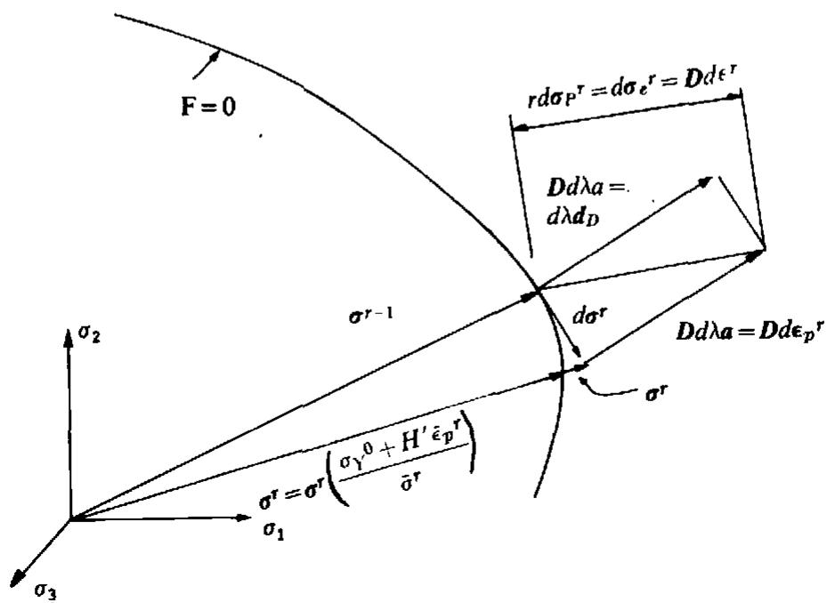
Step a. The applied loads for the $r^{\text{th}}$ iteration are the residual forces $\psi^{r-1}$ , given by (2.4) which give rise to displacement increments $dd^{r}$ , according to (2.12), and strain increments $d\epsilon^{r}$ .
Step b. Compute the incremental stress changes, $d\sigma_{e}^{r}$ as $d\sigma_{e}^{r} = Dd\varepsilon^{r}$ where the subscript e denotes that we are assuming elastic behaviour.
Step c. Accumulate the total stress for each element Gauss point as $\sigma_{e}^{r} = \sigma^{r-1} + d\sigma_{e}^{r}$ where $\sigma^{r-1}$ are the converged stresses for iteration r-1.
Step d. The next step depends on whether or not yielding took place at the Gauss point during the $(r-1)^{\text{th}}$ iteration. Therefore we check if $\bar{\sigma}^{r-1} > \sigma_{Y} = \sigma_{Y}^{\circ} + H' \bar{\epsilon}_{p}^{r-1}$ , where $\bar{\sigma}^{r-1}$ is the effective stress given by Column 3, Table 7.2, $\sigma_{Y}$ is the uniaxial yield stress, (Column 4, Table 7.2), $H'$ is the linear strain hardening parameter and $\bar{\epsilon}_{p}^{r-1}$ is the effective plastic strain existing at the end of the $(r-1)^{\text{th}}$ iteration. This expression is identical to the uniaxial case, Section 3.12.2, with all quantities replaced by the effective or equivalent values. If the answer is:
# YES
The Gauss point had previously yielded. Now check to see if $\bar{\sigma}_{e}^{r} > \bar{\sigma}^{r-1}$ where $\bar{\sigma}_{e}^{r}$ is the effective stress, Col. 3, Table 7.2 based on stresses $\sigma_{e}^{r}$ . If the answer is:
NO
YES
The Gauss point is unloading elastically and therefore go directly to Step g.
The Gauss point had yielded previously and the stress is still increasing. Therefore all the excess stress $\sigma_{e}^{r}-\sigma^{r-1}$ must be reduced to the yield surface as indicated in
Fig. 7.10(a). Therefore the factor R which defines the portion of stress which must be modified to satisfy the yield criterion is equal to 1.
# NO
Which implies that the Gauss point had not previously yielded. Now check to see if $\bar{\sigma}_{e}^{r} > \sigma_{Y}^{0}$ . If the answer is:
NO
YES
The Gauss point is still elastic and therefore go directly to Step g.
The Gauss point has yielded during application of load corresponding to this iteration as shown in
Fig. 7.10(b). The portion of the stress greater than the yield value must be reduced to the yield surface. The reduction factor R is given from
Fig. 7.10(b) to be
$$
R = \frac {A B}{A C} = \frac {\bar {\sigma} _ {e} ^ {r} - \sigma_ {Y}}{\bar {\sigma} _ {e} ^ {r} - \bar {\sigma} ^ {r - 1}}.
$$