text_image

reflection plane 8 7 7 + n 8 + n 5 6 6 + n 5 + n 4 3 c 3 + n 4 + n 2 + n 1 + n 1 2 a

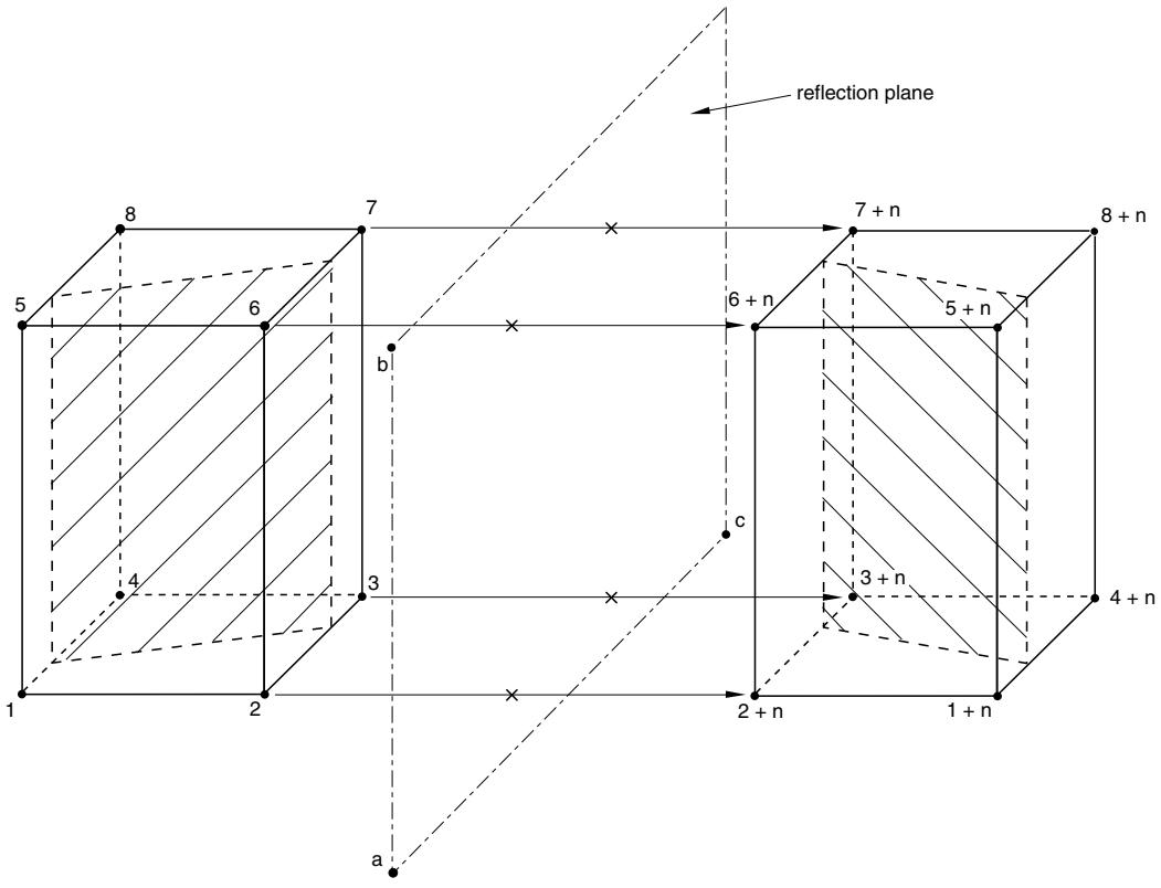
Figure 10.4.1–5 Reflecting a three-dimensional model through a plane with node offset n. Input File Usage: Use one of the following options: \*SYMMETRIC MODEL GENERATION, REFLECT=LINE \*SYMMETRIC MODEL GENERATION, REFLECT=PLANE # Controlling the new node and element numbering You can specify constants that must be added to the original node and element numbers for numbering the reflected part of the three-dimensional model. The defaults are the maximum node and element numbers used in the original model. Control over the numbering allows you to define additional parts of the model without the risk of conflicting element and node labels. Input File Usage: \*SYMMETRIC MODEL GENERATION, REFLECT, $\mathrm { N O D E ~ O F F S E T } = o f f s e t , \mathrm { E L E M E N T ~ O F F S E T } = o f f s e t$ # Limitations • Only surface-based contact pairs can be reflected. Models using general contact cannot be reflected. Contact conditions modeled with contact elements will be ignored in the model generation. • You must ensure that master surfaces remain continuous after reflection. A discontinuous surface is created when the surface in the original model does not intersect the connection plane between the two parts of the symmetric structure. • Rigid surfaces cannot be reflected. The rigid surface definition of the original model is simply repeated in the new model. You must, therefore, specify the complete rigid surface in the original model. • Most types of kinematic constraints cannot be reflected. However, surface-based constraints (“Mesh tie constraints,” Section 35.3.1) and embedded element constraints (“Embedded elements,” Section 35.4.1) defined in the original model will be generated automatically in the new three-dimensional model. • Only stress/displacement, heat transfer, coupled temperature-displacement, and acoustic elements can be reflected. • Nonaxisymmetric elements such as springs, dashpots, beams, and trusses cannot be reflected. # 10.4.2 TRANSFERRING RESULTS FROM A SYMMETRIC MESH OR A PARTIAL THREE-DIMENSIONAL MESH TO A FULL THREE-DIMENSIONAL MESH Product: Abaqus/Standard # References • “Symmetric model generation,” Section 10.4.1 • \*SYMMETRIC RESULTS TRANSFER # Overview Symmetric results transfer: • reduces the analysis cost of structures that may first undergo symmetric deformation followed by nonsymmetric deformation later during the loading history; • can be used to transfer the solution of an axisymmetric model to a three-dimensional model; • can be used to transfer the solution of the symmetric part of a three-dimensional model to a full three-dimensional model; • must be used in conjunction with the symmetric model generation capability (see “Symmetric model generation,” Section 10.4.1); and • can be used only to transfer the solution of a stress/displacement, heat transfer, coupled temperaturedisplacement, or coupled acoustic-structural analysis to a new model. # Transferring the solution from a symmetric mesh or a partial three-dimensional mesh to a full three-dimensional mesh The symmetric results transfer capability can be used to transfer the solution of an axisymmetric model to a three-dimensional model or to transfer the solution of the symmetric part of a three-dimensional model to a full three-dimensional model. The symmetric model generation capability described in “Symmetric model generation,” Section 10.4.1, must be used to generate the three-dimensional model. The symmetric results transfer capability is not available for models defined in terms of an assembly of part instances. The solution that is transferred to the new model consists of the deformed configuration and corresponding material state, which includes strains and all state variables. The nodes are imported with their original coordinates. This solution becomes the initial or base state in the new analysis. # Specifying the time at which the solution obtained in the original model must be read You specify the time at which the solution obtained in the original model must be read. The required step and increment or iteration must have been written to the restart files during the original analysis. # Input File Usage: Use the following option if the solution is transferred from any analysis other than a direct cyclic procedure: \*SYMMETRIC RESULTS TRANSFER, STEP=step, INC=increment Use the following option if the solution is transferred from a previous direct cyclic analysis: \*SYMMETRIC RESULTS TRANSFER, STEP=step, ITERATION=iteration # Obtaining equilibrium You must ensure that the model is in equilibrium at the beginning of the analysis. It is recommended that an initial step definition be included using boundary conditions and loading that match the state of the model from which the results are transferred. An initial time increment equal to the total time should be used for this step to allow Abaqus/Standard to try and achieve the equilibrium in one increment. If needed, Abaqus/Standard can resolve the stress unbalance linearly over the step such that more than one increment is used. You can choose to have the stress unbalance resolved in the first increment of the step instead. # Input File Usage: Use the following option to have Abaqus/Standard resolve the stress unbalance linearly over the step: \*SYMMETRIC RESULTS TRANSFER, UNBALANCED STRESS=RAMP Use the following option to have Abaqus/Standard resolve the stress unbalance in the first increment of the step: \*SYMMETRIC RESULTS TRANSFER, UNBALANCED STRESS=STEP # Identifying the restart files The symmetric results transfer capability uses the restart (.res), analysis database (.stt and .mdl), part (.prt), and output database (.odb) files from the old analysis to transfer the solution data to the new mesh. The name of the restart files from the old analysis must be specified when the new analysis is executed by using the oldjob parameter in the command for running Abaqus or by answering a request made by the command procedure (see “Abaqus/Standard, Abaqus/Explicit, and Abaqus/CFD execution,” Section 3.2.2). # Verifying the new model It is recommended that you verify that the new model is generated correctly before results are transferred or any analysis is performed. The model generation capability requires only information stored in the restart files during a data check run to generate the new model, which allows you to verify the new model before the analysis of the original model is performed. A data check analysis is performed by using the datacheck parameter in the command for running Abaqus (see “Abaqus/Standard, Abaqus/Explicit, and Abaqus/CFD execution,” Section 3.2.2). Once the model has been verified, the analysis of the original model can be performed and the results can be transferred to the new model. The transferred solution can be written to the results files by requesting output at the beginning of a step (the zero increment; see “Output,” Section 4.1.1). This solution can also be viewed in Abaqus/CAE. # Orientation system When results are transferred from an axisymmetric model to a three-dimensional model, a local cylindrical orientation system is used for element output of stress, strain, etc. A default local orientation definition (“Orientations,” Section 2.2.5) is provided if the material in the original axisymmetric model does not contain an orientation definition. This default orientation is defined with the polar axis of the system along the axis of revolution with an additional 90° rotation about the local 1-direction so that the local axes are 1=radial, 2=axial, and 3=circumferential. If shells or membranes are used, the projections of the local 2- and 3-axes onto the surface of the shell or membrane are taken as the local directions on the surface. It is assumed that the material properties are specified in this system. If, on the other hand, an orientation definition is associated with the material in the original model, the orientation in the new three-dimensional model will be that orientation definition revolved about the axis of symmetry. When results are transferred from a partial three-dimensional model to a full three-dimensional model by reflecting the partial three-dimensional model, a local material orientation is created in the full three-dimensional model based on the corresponding orientation definition in the partial three-dimensional model. However, if the material does not contain an orientation definition in the partial three-dimensional model and the partial three-dimensional model is not created by revolving an axisymmetric model, no local orientation definition is created in the full three-dimensional model. The full three-dimensional model uses a global coordinate system. When results are transferred from a three-dimensional sector to a periodic three-dimensional model by revolving the three-dimensional sector about its symmetry axis, a local cylindrical orientation system is always used for element output of stress, strain, etc. If an orientation is specified in the original three-dimensional sector, the orientation system in the new model is defined by revolving the original orientation system about the symmetry axis. If shells or membranes are used, the projections of the local 2- and 3-axes onto the surface of the shell or membrane are taken as the local directions on the surface. If the material in the original three-dimensional sector does not contain an orientation definition, a default local orientation definition is provided. This default orientation is defined by revolving the global coordinate system in the original model about the axis of symmetry in the new model. # Coordinate system at nodes The displacement and rotational components obtained from the original model are first transformed into a global, rectangular Cartesian axis system before the results are transferred. If local coordinate directions are required in the new model, a nodal transformation (“Transformed coordinate systems,” Section 2.1.5) must be specified in the new model to define this coordinate system. # Limitations The following limitations exist for result transfer from an axisymmetric model to a 3D model: • Result transfer is not available from 8-node reduced-integration axisymmetric elements (CAX8R and CAX8RH) to the corresponding 20-node brick elements (C3D20R and C3D20RH) when the elements are underlying the slave surface in a contact pair. • SAX2 is a finite-strain shell, while S8R is a small-strain shell. Do not use this combination when deformations are large in the original analysis. The following limitation exists for result transfer from a symmetric 3D model to a full 3D model: • Result transfer is not supported for shells with five degrees of freedom per node (STRI65, S8R5, and S9R5). # Initial conditions Initial conditions (see “Initial conditions in Abaqus/Standard and Abaqus/Explicit,” Section 34.2.1) can be specified on all nodes and elements, including the part of the model generated using symmetric model generation (see “Symmetric model generation,” Section 10.4.1). However, in most cases the symmetric results transfer capability will overwrite the initial condition values with the solution obtained from the original model. An exception is initial temperatures and field variables. Initial temperatures and field variables are overwritten only when temperatures and field variables are specified in the original model. If only part of the original model contains a specification for temperatures or field variables, the remaining part of the model is assumed to have initial conditions with a magnitude of zero. This distribution of the field will be transferred to the new model. If temperatures and/or field variables are not defined anywhere in the original model, the initial conditions specified in the new model are applied. # Boundary conditions All boundary conditions must be redefined; the symmetric result transfer capability ignores the boundary conditions specified in the original model. You must ensure that the model is in equilibrium at the beginning of the analysis; therefore, an initial step definition should be included using boundary conditions and loading that match the state of the model from which the results are transferred. # Loads All loads must be redefined; the symmetric result transfer capability ignores the loads specified in the original model. You must ensure that the model is in equilibrium at the beginning of the analysis; therefore, an initial step definition should be included using boundary conditions and loading that match the state of the model from which the results are transferred. # Material options All of the material definitions defined in the original model will be transferred to the new model. # Elements Any element or contact pair removal/reactivation definition (see “Element and contact pair removal and reactivation,” Section 11.2.1) that was active in the original model should be respecified. # Output All of the standard output variables available for stress/displacement elements can be used with the symmetric results transfer capability. The solution that is transferred to the new model can be written to the results (.fil) file by requesting output at the beginning of a step (the zero increment; see “Output,” Section 4.1.1). It can also be displayed in Abaqus/CAE. # 10.4.3 ANALYSIS OF MODELS THAT EXHIBIT CYCLIC SYMMETRY Products: Abaqus/Standard Abaqus/CAE # References • “Natural frequency extraction,” Section 6.3.5 • “Mode-based steady-state dynamic analysis,” Section 6.3.8 • \*CYCLIC SYMMETRY MODEL • \*SELECT CYCLIC SYMMETRY MODES • \*SURFACE • \*TIE • “Defining cyclic symmetry,” Section 15.13.19 of the Abaqus/CAE User’s Guide, in the HTML version of this guide # Overview The cyclic symmetry analysis technique in Abaqus/Standard: • makes it possible to analyze the behavior of a $3 6 0 ^ { \circ }$ structure with cyclic symmetry based on a model of a repetitive sector; • can determine the response to cyclic symmetric loading in static, quasi-static, and heat transfer analyses; • can calculate all eigenfrequencies and eigenmodes of the 360° structure with the block Lanczos eigenfrequency extraction procedure; • can determine the response to loading corresponding to a given cyclic symmetry mode in modalbased steady-state dynamic analysis; and • does not require that matched meshes be used on the symmetry surfaces. # Introduction Structures that exhibit cyclic symmetry provide the analyst with an opportunity to model an entire 360° structure at considerably reduced computational expense by analyzing only a single repetitive sector of the model. Typically, this is the smallest sector that can be identified, although this is not necessary. For example, if a structure consists of 16 repetitive sectors it is possible to use a $4 5 ^ { \circ }$ model containing two repetitive sectors. The sectors are numbered in the counterclockwise direction to the axis of cyclic symmetry (as described further below). Of course this is less efficient than using a 22.5° model with one sector. There is no restriction that the meshes on the two symmetry surfaces of a repetitive sector match in any way. There are two basic cases that must be considered in such an analysis: a model that has a cyclic symmetric initial state and a cyclic symmetric response, and a model with a cyclic symmetric initial state but a nonsymmetric response. The cyclic symmetry capability in Abaqus/Standard provides for linear and nonlinear analysis of cyclic symmetric structures with cyclic symmetric response. The condition that the structure be cyclic symmetric holds throughout the analysis, so in a loading step it is not possible to have any nonsymmetric deformation in the structure at any time. Therefore, only cyclic symmetric loads can be applied for this situation. 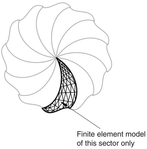Analysis of cyclic symmetric structures that exhibit nonsymmetric response requires additional consideration. Such an analysis can be performed only in a linear perturbation step, since the nonsymmetric deformation invalidates the assumption of a cyclic symmetric “base state” for any subsequent step in a general nonlinear analysis. The full response of an entire cyclic symmetric structure, such as the structure illustrated in Figure 10.4.3–1, can be represented as a linear combination of several independent basic responses, each of which corresponds to some k-fold cyclic symmetry mode. 

text_image

Finite element model of this sector only

Figure 10.4.3–1 Cyclic symmetric structure. The cyclic symmetry mode number, which is sometimes also referred to as the “nodal diameter,” indicates the number of waves along the circumference in a basic response. Figure 10.4.3–2, Figure 10.4.3–3, and Figure 10.4.3–4 illustrate basic responses corresponding to the 0-, 1-, and 2-fold modes (nodal diameters 0, 1, and 2) in a cyclic symmetric structure containing four repetitive sectors. A full linear perturbation analysis can be performed by solving a sequence of corresponding linear analyses for a symmetric single sector. Cyclic symmetric boundary conditions (associated with various cyclic symmetry modes) on the single sector give rise to Hermitian stiffness and mass matrices (complex matrices with symmetric real parts and skew-symmetric imaginary parts). The kth linear analysis in the sequence is performed using symmetry conditions that correspond to the k-fold cyclic symmetry mode of the structural response. For a structure exhibiting N-fold cyclic symmetry, only (N even) or (N odd) such analyses are required. This results in a solution for the response of the entire structure at a relatively low computational expense.