| $\bar{I}_{1}$ | is the first invariant of $\bar{\mathbf{B}}$ , |
| $\bar{I}_{2}$ | is the second invariant of $\bar{\mathbf{B}}$ , |
| $\dot{\bar{\varepsilon}}^{cr}$ , $\bar{\varepsilon}^{cr}$ , $J$ , $p$ and $\tilde{q}$ | are defined above, |
| $t$ | is the time, |
| $\theta$ | is the temperature, and |
| $FV$ | are field variables. |
The tensor is defined in “UCREEPNETWORK,” Section 1.1.23 of the Abaqus User Subroutines Reference Guide.
# Thermal expansion
Only isotropic thermal expansion is permitted with nonlinear viscoelastic materials (“Thermal expansion,” Section 26.1.2).
# Defining viscoelastic response
The nonlinear viscoelastic response is defined by specifying the identifier, stiffness ratio, and creep law for each viscoelastic network.
# Specifying network identifier
Each viscoelastic network in the material model must be assigned a unique network identifier or network id. The network identifiers must be consecutive integers starting with 1. The order in which they are specified is not important.
Input File Usage: Use the following option to specify the network identifier:
$* \mathrm { V I S C O E L A S T I C } , \mathrm { N O N L I N E A R } , \mathrm { N E T W O R K I D } = n e t w o r k I d$
# Defining the stiffness ratio
The contribution of each network to the overall response of the material is determined by the value of the stiffness ratio, , which is used to scale the elastic response of the network material. The sum of the stiffness ratios of the viscoelastic networks must be smaller than or equal to 1. If the sum of the ratios is equal to 1, the purely elastic equilibrium network is not created. If the sum of the ratios is smaller than 1, the equilibrium network is created with a stiffness ratio, $r _ { 0 }$ , equal to
$$
r _ {0} = 1 - \sum_ {k = 1} ^ {N} r _ {k},
$$
where denotes the number of viscoelastic networks and $r _ { k }$ is the stiffness ratio of network . You can specify the stiffness ratio to remain constant during the analysis or to vary as a function of temperature and predefined field variables.
Defining a constant stiffness ratio
You can specify that the stiffness ratio remains constant during the analysis:
Input File Usage: \*VISCOELASTIC, NONLINEAR, SRATIO=ratio
Defining a temperature- and field-variable dependent stiffness ratio
Alternatively, you can define the stiffness ratio as a function of temperature and predefined field variables.
Input File Usage: \*NETWORK STIFFNESS RATIO, N=nNetworks, DEPENDENCIES=n
# Specifying the creep law
The definition of creep behavior in Abaqus/Standard is completed by specifying the creep law.
Power law creep model
The power law model is defined by specifying five material parameters: , n, m, a, and $\dot { \varepsilon } _ { 0 }$ . The parameter $\dot { \varepsilon } _ { 0 }$ must be positive. It is introduced for dimensional consistency, and its default value is 1.0. For physically reasonable behavior $q _ { 0 }$ and n must be positive, a must be nonnegative (the default is 0.0), and $- 1 < m \leq 0$ .
Input File Usage: \*VISCOELASTIC, NONLINEAR, LAW=POWER LAW
Strain hardening power law creep model
The strain hardening law is defined by specifying three material parameters: A, n, and m. For physically reasonable behavior A and n must be positive and $- 1 < m \leq 0$ .
Input File Usage: \*VISCOELASTIC, NONLINEAR, LAW=STRAIN
Hyperbolic sine creep model
The hyperbolic sine creep law is specified by providing three nonnegative parameters: A, B, and n.
Input File Usage: \*VISCOELASTIC, NONLINEAR, LAW=HYPERB
Bergstrom-Boyce creep model
The Bergstrom-Boyce creep law is specified by providing four parameters: A, m, C, and E. The parameters A and E must be nonnegative, the parameter m must be positive, and the parameter C must lie in .
Input File Usage: \*VISCOELASTIC, NONLINEAR, LAW=BERGSTROM-BOYCE
User-defined creep model
An alternative method for defining the creep law involves using user subroutine UCREEPNETWORK in Abaqus/Standard or VUCREEPNETWORK in Abaqus/Explicit. Optionally, you can specify the number of property values needed as data in the user subroutine.
Input File Usage: \*VISCOELASTIC, NONLINEAR, LAW=USER, PROPERTIES=n
Numerical difficulties
Depending on the choice of units, the value of A in the strain power-law, hyperbolic-sine, and Bergstrom-Boyce models may be very small for typical creep strain rates. If A is less than $1 0 ^ { - 2 7 }$ , numerical difficulties can cause errors in the material calculations; therefore, a different system of units should be used to avoid such difficulties in the calculation of creep strain increments. In such cases it is recommended to replace the strain power-law model with the power law model, which does not have the limitation described above. The strain power-law model is a special case of the power law model obtained by setting , , and $q _ { 0 } = A ^ { - 1 / n }$ .
# Thermo-rheologically simple temperature effects
Thermo-rheologically simple temperature effects can be included for each viscoelastic network. In this case the creep law is modified and takes the following form:
$$
\frac {d \bar {\varepsilon} ^ {c r}}{d \tau} = \frac {1}{a _ {T} (\theta)} g ^ {c r} (\bar {\varepsilon} ^ {c r}, I _ {1} ^ {c r}, \bar {I} _ {1}, \bar {I} _ {2}, J, p, \tilde {q}, \tau),
$$
where and $a _ { T } ( \theta )$ denote the reduced time and the shift function, respectively. The reduced time is related to the actual time through the integral differential equation
$$
\tau = \int_ {0} ^ {t} \frac {d t ^ {\prime}}{a _ {T} (\theta)}, \qquad \frac {d \tau}{d t} = \frac {1}{a _ {T} (\theta)}.
$$
Abaqus supports the following forms of the shift function: the Williams-Landel-Ferry (WLF) form and the Arrhenius form (see “Thermo-rheologically simple temperature effects” in “Time domain viscoelasticity,” Section 22.7.1). In addition, user-defined forms can be specified in Abaqus/Standard.
# User-defined form in Abaqus/Standard
An alternative method for specifying the shift function involves using user subroutine UTRSNETWORK. Optionally, you can specify the number of property values needed as data in the user subroutine.
Input File Usage: \*TRS, DEFINITION=USER, PROPERTIES=n
# Material response in different analysis steps
In Abaqus/Standard the material is active during all stress/displacement procedure types. However, the creep effects are taken into account only in quasi-static (“Quasi-static analysis,” Section 6.2.5), coupled temperature-displacement (“Fully coupled thermal-stress analysis,” Section 6.5.3), direct-integration implicit dynamic (“Implicit dynamic analysis using direct integration,” Section 6.3.2), and steady-state transport (“Steady-state transport analysis,” Section 6.4.1) analyses. If the material is used in a steady-state transport analysis, it cannot include plasticity. In other stress/displacement procedures the evolution of the state variables is suppressed and the creep strain remains unchanged. In Abaqus/Explicit the creep effects are always active.
# Elements
The nonlinear viscoelastic model is available with continuum elements that include mechanical behavior (elements that have displacement degrees of freedom), except for one-dimensional and plane stress elements.
# Output
In addition to the standard output identifiers available in Abaqus (“Abaqus/Standard output variable identifiers,” Section 4.2.1, and “Abaqus/Explicit output variable identifiers,” Section 4.2.2), the following variables have special meaning for the nonlinear viscoelastic material model:
CEEQ $\begin{array} { r } { \bar { \varepsilon } ^ { c r } = \sum _ { k = 1 } ^ { N } r _ { k } \bar { \varepsilon } _ { k } ^ { c r } } \end{array}$
CE The overall creep strain, defined as $\begin{array} { r } { \varepsilon ^ { c r } = \sum _ { k = 1 } ^ { N } r _ { k } \varepsilon _ { k } ^ { c r } } \end{array}$
CENER The overall viscous dissipated energy per unit volume, defined as $\begin{array} { r } { E _ { c } = \sum _ { k = 1 } ^ { N } E _ { c } ^ { k } } \end{array}$
SENER $\begin{array} { r } { E _ { s } = \sum _ { k = 0 } ^ { N } E _ { s } ^ { k } } \end{array}$ astic strain energy density per unit volume, defined as.
SNETk All stress components in the $k ^ { t h }$ network $( 0 \leq k \leq 1 0 )$
In the above definitions $r _ { k }$ denotes the stiffness ratio for network , denotes the number of viscoelastic networks, the subscript or superscript is used to denote network quantities, and the network is assumed to be the purely elastic network.
If plasticity is specified in the equilibrium network, the standard output identifiers available in Abaqus corresponding to other isotropic and kinematic hardening plasticity models can be obtained for this model as well. In addition, if the Mullins effect is used in the model, the output variables available for the Mullins effect model (see “Mullins effect,” Section 22.6.1) can be requested.
# Additional references
• Bergstrom, J. S., and M. C. Boyce, “Constitutive Modeling of the Large Strain Time-Dependent Behavior of Elastomers,” Journal of the Mechanics and Physics of Solids, vol. 46, pp. 931–954, 1998.
• Bergstrom, J. S., and M. C. Boyce, “Large Strain Time-Dependent Behavior of Filled Elastomers,” Mechanics of Materials, vol. 32, pp. 627–644, 2000.
• Bergstrom, J. S., and J. E. Bischoff, “An Advanced Thermomechanical Constitutive Model for UHMWPE,” International Journal of Structural Changes in Solids, vol. 2, pp. 31–39, 2010.
• Hurtado, J. A., I. Lapczyk, and S. M. Govindarajan, “Parallel Rheological Framework to Model Non-Linear Viscoelasticity, Permanent Set, and Mullins Effect in Elastomers,” Constitutive Models for Rubber VIII, p. 95, 2013.
• Lapczyk, I., J. A. Hurtado, and S. M. Govindarajan, “A Parallel Rheological Framework for Modeling Elastomers and Polymers,” 182nd Technical Meeting of the Rubber Division of the American Chemical Society, pp. 1840–1859, October 2012, Cincinnati, OH.
# 22.9 Rate sensitive elastomeric foams
• “Low-density foams,” Section 22.9.1
# 22.9.1 LOW-DENSITY FOAMS
Products: Abaqus/Explicit Abaqus/CAE
# References
• “Material library: overview,” Section 21.1.1
• “Elastic behavior: overview,” Section 22.1.1
• \*LOW DENSITY FOAM
• \*UNIAXIAL TEST DATA
• “Creating a low-density foam material model” in “Defining elasticity,” Section 12.9.1 of the Abaqus/CAE User’s Guide, in the HTML version of this guide
# Overview
The low-density foam material model:
• is intended for low-density, highly compressible elastomeric foams with significant rate sensitive behavior (such as polyurethane foam);
• requires the direct specification of uniaxial stress-strain curves at different strain rates for both tension and compression;
• optionally allows the specification of lateral strain data to include Poisson effects;
• allows for the specification of optional unloading stress-strain curves for better representation of the hysteretic behavior and energy absorption during cyclic loading; and
• requires that geometric nonlinearity be accounted for during the analysis step (see “Defining an analysis,” Section 6.1.2, and “General and linear perturbation procedures,” Section 6.1.3), since it is intended for finite-strain applications.
# Mechanical response
Low-density, highly compressible elastomeric foams are widely used in the automotive industry as energy absorbing materials. Foam padding is used in many passive safety systems, such as behind headliners for head impact protection, in door trims for pelvis and thorax protection, etc. Energy absorbing foams are also commonly used in packaging of hand-held and other electronic devices.
The low-density foam material model in Abaqus/Explicit is intended to capture the highly strain-rate sensitive behavior of these materials. The model uses a pseudo visco-hyperelastic formulation whereby the strain energy potential is constructed numerically as a function of principal stretches and a set of internal variables associated with strain rate. By default the Poisson’s ratio of the material is assumed to be zero. With this assumption, the evaluation of the stress-strain response becomes uncoupled along the principal deformation directions. Optionally, nonzero Poisson effects can be specified to include coupling along the principal directions.
The model requires as input the stress-strain response of the material for both uniaxial tension and uniaxial compression tests. Poisson effects can be included by also specifying lateral strain data for each of these tests. The tests can be performed at different strain rates. For each test the strain data should be given in nominal strain values (change in length per unit of original length), and the stress data should be given in nominal stress values (force per unit of original cross-sectional area). Uniaxial tension and compression curves are specified separately. The uniaxial stress and strain data are given in absolute values (positive in both tension and compression). On the other hand, when specified, the lateral strain data must be negative in tension and positive in compression, corresponding to a positive Poisson’s effect. The model does not support negative Poisson’s effect. Rate-dependent behavior is specified by providing the uniaxial stress-strain curves for different values of nominal strain rates.
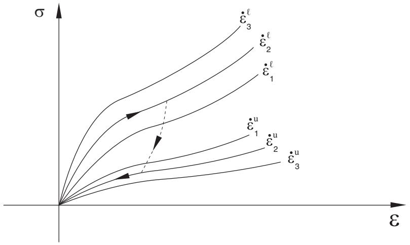
Both loading and unloading rate-dependent curves can be specified to better characterize the hysteretic behavior and energy absorption properties of the material during cyclic loading. Use positive values of nominal strain rates for loading curves and negative values for the unloading curves. Currently this option is available only with linear strain rate regularization (see “Regularization of strain-rate-dependent data in Abaqus/Explicit” in “Material data definition,” Section 21.1.2). When the unloading behavior is not specified directly, the model assumes that unloading occurs along the loading curve associated with the smallest deformation rate. A representative schematic of typical rate-dependent uniaxial compression data is shown in Figure 22.9.1–1 with both loading and unloading curves. It is important that the specified rate-dependent stress-strain curves do not intersect. Otherwise, the material is unstable, and Abaqus issues an error message if an intersection between curves is found.