text_image

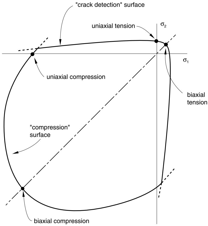
"crack detection" surface uniaxial tension σ₂ σ₁ uniaxial compression "compression" surface biaxial tension

Figure 23.6.1–4 Yield and failure surfaces in plane stress. • The ratio of the tensile principal stress at cracking, in plane stress, when the other principal stress is at the ultimate compressive value, to the tensile cracking stress under uniaxial tension. Default values of the above ratios are used if you do not specify them. Input File Usage: \*FAILURE RATIOS Abaqus/CAE Usage: Property module: material editor: Mechanical→Plasticity→Concrete Smeared Cracking: Suboptions→Failure Ratios # Response to strain reversals Because the model is intended for application to problems involving relatively monotonic straining, no attempt is made to include prediction of cyclic response or of the reduction in the elastic stiffness caused 

line

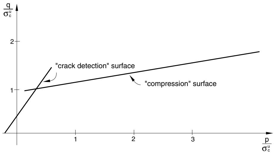
| p/σ_c^u | q/σ_c^u (crack detection) | q/σ_c^u (compression) | | ------- | -------------------------- | ---------------------- | | 0 | 0 | 0 | | 1 | 1 | 1 | | 2 | 1.5 | 1.5 | | 3 | 2 | 2 |

Figure 23.6.1–5 Yield and failure surfaces in the (p–q) plane. by inelastic straining under predominantly compressive stress. Nevertheless, it is likely that, even in those applications for which the model is designed, the strain trajectories will not be entirely radial, so that the model should predict the response to occasional strain reversals and strain trajectory direction changes in a reasonable way. Isotropic hardening of the “compressive” yield surface forms the basis of this aspect of the model’s inelastic response prediction when the principal stresses are dominantly compressive. # Calibration A minimum of two experiments, uniaxial compression and uniaxial tension, is required to calibrate the simplest version of the concrete model (using all possible defaults and assuming temperature and field variable independence). Other experiments may be required to gain accuracy in postfailure behavior. # Uniaxial compression and tension tests The uniaxial compression test involves compressing the sample between two rigid platens. The load and displacement in the direction of loading are recorded. From this, you can extract the stress-strain curve required for the concrete model directly. The uniaxial tension test is much more difficult to perform in the sense that it is necessary to have a stiff testing machine to be able to record the postfailure response. Quite often this test is not available, and you make an assumption about the tensile failure strength of the concrete (usually about 7%–10% of the compressive strength). The choice of tensile cracking stress is important; numerical problems may arise if very low cracking stresses are used (less than 1/100 or 1/1000 of the compressive strength). # Postcracking tensile behavior The calibration of the postfailure response depends on the reinforcement present in the concrete. For plain concrete simulations the stress-displacement tension stiffening model should be used. Typical values for $u _ { 0 }$ are 0.05 mm $( 2 \times 1 0 ^ { - 3 }$ in) for a normal concrete to 0.08 mm $( 3 \times 1 0 ^ { - 3 }$ in) for a high-strength concrete. For reinforced concrete simulations the stress-strain tension stiffening model should be used. A reasonable starting point for relatively heavily reinforced concrete modeled with a fairly detailed mesh is to assume that the strain softening after failure reduces the stress linearly to zero at a total strain of about 10 times the strain at failure. Since the strain at failure in standard concretes is typically $1 0 ^ { - 4 }$ , this suggests that tension stiffening that reduces the stress to zero at a total strain of about $1 0 ^ { - 3 }$ is reasonable. This parameter should be calibrated to a particular case. # Postcracking shear behavior Combined tension and shear experiments are used to calibrate the postcracking shear behavior in Abaqus/Standard. These experiments are quite difficult to perform. If the test data are not available, a reasonable starting point is to assume that the shear retention factor, , goes linearly to zero at the same crack opening strain used for the tension stiffening model. # Biaxial yield and flow parameters Biaxial experiments are required to calibrate the biaxial yield and flow parameters used to specify the failure ratios. If these are not available, the defaults can be used. # Temperature dependence The calibration of temperature dependence requires the repetition of all the above experiments over the range of interest. 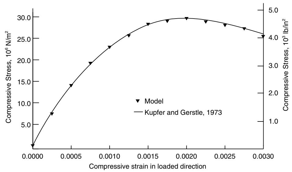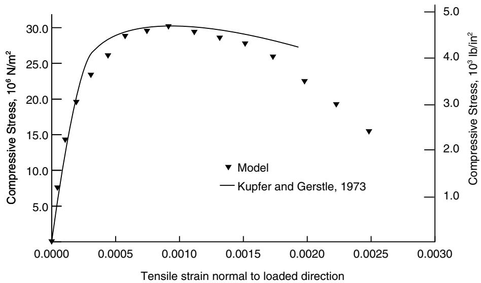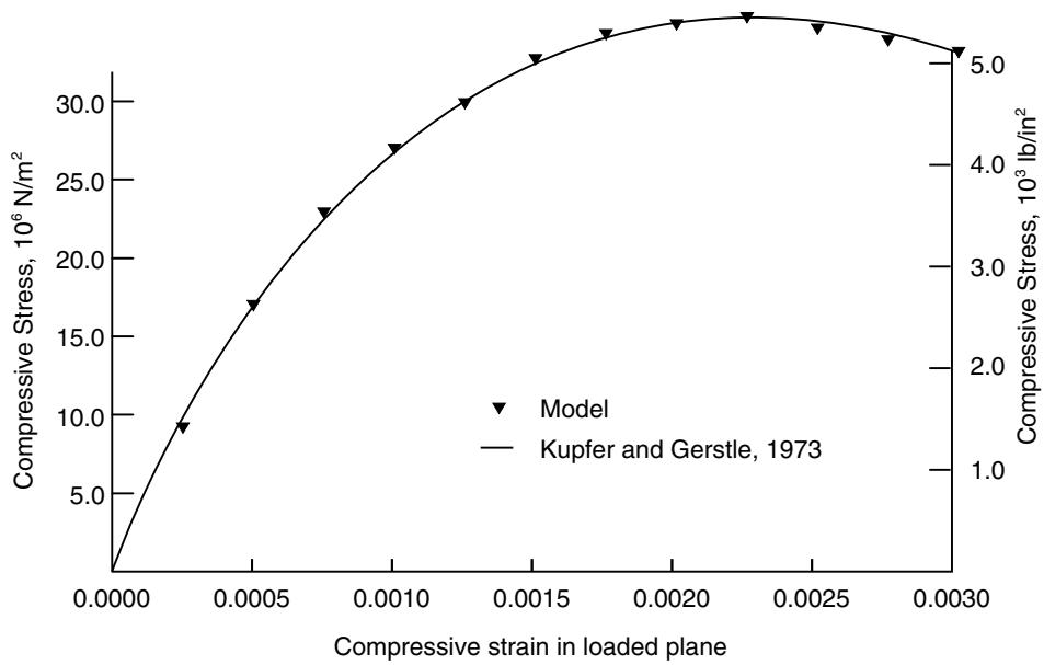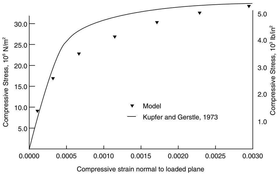# Comparison with experimental results With proper calibration, the concrete model should produce reasonable results for mostly monotonic loadings. Comparison of the predictions of the model with the experimental results of Kupfer and Gerstle (1973) are shown in Figure 23.6.1–6 and Figure 23.6.1–7. # Elements Abaqus/Standard offers a variety of elements for use with the smeared crack concrete model: beam, shell, plane stress, plane strain, generalized plane strain, axisymmetric, and three-dimensional elements. For general shell analysis more than the default number of five integration points through the thickness of the shell should be used; nine thickness integration points are commonly used to model progressive failure of the concrete through the thickness with acceptable accuracy.  

bar_line

| Tensile strain normal to loaded direction | Compressive Stress, 10⁶ N/m² | Compressive Stress, 10³ lb/in² | | ----------------------------------------- | ----------------------------- | ------------------------------ | | 0.0000 | 0.0 | 0.0 | | 0.0002 | 14.0 | 1.0 | | 0.0004 | 20.0 | 2.0 | | 0.0006 | 26.0 | 3.0 | | 0.0008 | 29.0 | 4.0 | | 0.0010 | 30.0 | 4.5 | | 0.0012 | 29.0 | 4.5 | | 0.0014 | 28.0 | 4.5 | | 0.0016 | 27.0 | 4.5 | | 0.0018 | 26.0 | 4.5 | | 0.0020 | 23.0 | 4.0 | | 0.0022 | 19.0 | 3.0 | | 0.0024 | 15.0 | 2.0 | | 0.0026 | 10.0 | 1.0 | | 0.0028 | 5.0 | 0.0 |

Figure 23.6.1–6 Comparison of model prediction and Kupfer and Gerstle’s data for a uniaxial compression test. 

line

| Compressive strain in loaded plane | Compressive Stress, 10⁶ N/m² | Compressive Stress, 10³ lb/in² | | ---------------------------------- | ----------------------------- | ------------------------------ | | 0.0000 | 0.0 | 0.0 | | 0.0005 | 10.0 | 1.0 | | 0.0010 | 20.0 | 2.0 | | 0.0015 | 25.0 | 3.0 | | 0.0020 | 30.0 | 4.0 | | 0.0025 | 30.0 | 5.0 | | 0.0030 | 30.0 | 5.0 |


bar_line

| Compressive strain normal to loaded plane | Compressive Stress, 10⁶ N/m² | Compressive Stress, 10³ lb/in² | | ---------------------------------------- | ----------------------------- | ------------------------------ | | 0.0000 | 9.0 | 1.0 | | 0.0005 | 17.0 | 2.5 | | 0.0010 | 23.0 | 3.5 | | 0.0015 | 27.0 | 4.0 | | 0.0020 | 30.0 | 4.5 | | 0.0025 | 32.0 | 4.8 | | 0.0030 | 33.0 | 5.0 |

Figure 23.6.1–7 Comparison of model prediction and Kupfer and Gerstle’s data for a biaxial compression test. # Output In addition to the standard output identifiers available in Abaqus/Standard (“Abaqus/Standard output variable identifiers,” Section 4.2.1), the following variables relate specifically to material points in the smeared crack concrete model: CRACK Unit normal to cracks in concrete. CONF Number of cracks at a concrete material point. # Additional references • Crisfield, M. A., “Snap-Through and Snap-Back Response in Concrete Structures and the Dangers of Under-Integration,” International Journal for Numerical Methods in Engineering, vol. 22, pp. 751–767, 1986. • Hillerborg, A., M. Modeer, and P. E. Petersson, “Analysis of Crack Formation and Crack Growth in Concrete by Means of Fracture Mechanics and Finite Elements,” Cement and Concrete Research, vol. 6, pp. 773–782, 1976. • Kupfer, H. B., and K. H. Gerstle, “Behavior of Concrete under Biaxial Stresses,” Journal of Engineering Mechanics Division, ASCE, vol. 99, p. 853, 1973. # 23.6.2 CRACKING MODEL FOR CONCRETE Products: Abaqus/Explicit Abaqus/CAE # References • “Material library: overview,” Section 21.1.1 • “Inelastic behavior,” Section 23.1.1 • \*BRITTLE CRACKING • \*BRITTLE FAILURE • \*BRITTLE SHEAR • “Defining brittle cracking” in “Defining other mechanical models,” Section 12.9.4 of the Abaqus/CAE User’s Guide, in the HTML version of this guide # Overview The brittle cracking model in Abaqus/Explicit: • provides a capability for modeling concrete in all types of structures: beams, trusses, shells and solids; • can also be useful for modeling other materials such as ceramics or brittle rocks; • is designed for applications in which the behavior is dominated by tensile cracking; • assumes that the compressive behavior is always linear elastic; • must be used with the linear elastic material model (“Linear elastic behavior,” Section 22.2.1), which also defines the material behavior completely prior to cracking; • is most accurate in applications where the brittle behavior dominates such that the assumption that the material is linear elastic in compression is adequate; • can be used for plain concrete, even though it is intended primarily for the analysis of reinforced concrete structures; • allows removal of elements based on a brittle failure criterion; and • is defined in detail in “A cracking model for concrete and other brittle materials,” Section 4.5.3 of the Abaqus Theory Guide. See “Inelastic behavior,” Section 23.1.1, for a discussion of the concrete models available in Abaqus. # Reinforcement Reinforcement in concrete structures is typically provided by means of rebars. Rebars are one-dimensional strain theory elements (rods) that can be defined singly or embedded in oriented surfaces. Rebars are discussed in “Defining rebar as an element property,” Section 2.2.4. They are typically used with elastic-plastic material behavior and are superposed on a mesh of standard element types used to model the plain concrete. With this modeling approach, the concrete cracking behavior is considered independently of the rebar. Effects associated with the rebar/concrete interface, such as bond slip and dowel action, are modeled approximately by introducing some “tension stiffening” into the concrete cracking model to simulate load transfer across cracks through the rebar. # Cracking Abaqus/Explicit uses a smeared crack model to represent the discontinuous brittle behavior in concrete. It does not track individual “macro” cracks: instead, constitutive calculations are performed independently at each material point of the finite element model. The presence of cracks enters into these calculations by the way in which the cracks affect the stress and material stiffness associated with the material point. For simplicity of discussion in this section, the term “crack” is used to mean a direction in which cracking has been detected at the single material calculation point in question: the closest physical concept is that there exists a continuum of micro-cracks in the neighborhood of the point, oriented as determined by the model. The anisotropy introduced by cracking is assumed to be important in the simulations for which the model is intended. # Crack directions The Abaqus/Explicit cracking model assumes fixed, orthogonal cracks, with the maximum number of cracks at a material point limited by the number of direct stress components present at that material point of the finite element model (a maximum of three cracks in three-dimensional, plane strain, and axisymmetric problems; two cracks in plane stress and shell problems; and one crack in beam or truss problems). Internally, once cracks exist at a point, the component forms of all vector- and tensor-valued quantities are rotated so that they lie in the local system defined by the crack orientation vectors (the normals to the crack faces). The model ensures that these crack face normal vectors will be orthogonal, so that this local crack system is rectangular Cartesian. For output purposes you are offered results of stresses and strains in the global and/or local crack systems. # Crack detection A simple Rankine criterion is used to detect crack initiation. This criterion states that a crack forms when the maximum principal tensile stress exceeds the tensile strength of the brittle material. Although crack detection is based purely on Mode I fracture considerations, ensuing cracked behavior includes both Mode I (tension softening/stiffening) and Mode II (shear softening/retention) behavior, as described later. As soon as the Rankine criterion for crack formation has been met, we assume that a first crack has formed. The crack surface is taken to be normal to the direction of the maximum tensile principal stress. Subsequent cracks may form with crack surface normals in the direction of maximum principal tensile stress that is orthogonal to the directions of any existing crack surface normals at the same point. Cracking is irrecoverable in the sense that, once a crack has occurred at a point, it remains throughout the rest of the calculation. However, crack closing and reopening may take place along the directions of the crack surface normals. The model neglects any permanent strain associated with cracking; that is, it is assumed that the cracks can close completely when the stress across them becomes compressive. You can specify the postfailure behavior for direct straining across cracks by means of a postfailure stress-strain relation or by applying a fracture energy cracking criterion. # Postfailure stress-strain relation In reinforced concrete the specification of postfailure behavior generally means giving the postfailure stress as a function of strain across the crack (Figure 23.6.2–1). In cases with little or no reinforcement, this introduces mesh sensitivity in the results, in the sense that the finite element predictions do not converge to a unique solution as the mesh is refined because mesh refinement leads to narrower crack bands. 

line

| e_nn^ck | σ_t^I | | ------- | ----- | | 0 | 1.0 | | 1 | 0.5 | | 2 | 0.3 | | 3 | 0.2 | | 4 | 0.1 |

Figure 23.6.2–1 Postfailure stress-strain curve. In practical calculations for reinforced concrete, the mesh is usually such that each element contains rebars. In this case the interaction between the rebars and the concrete tends to mitigate this effect, provided that a reasonable amount of “tension stiffening” is introduced in the cracking model to simulate this interaction. This requires an estimate of the tension stiffening effect, which depends on factors such as the density of reinforcement, the quality of the bond between the rebar and the concrete, the relative size of the concrete aggregate compared to the rebar diameter, and the mesh. A reasonable starting point for relatively heavily reinforced concrete modeled with a fairly detailed mesh is to assume that the strain softening after failure reduces the stress linearly to zero at a total strain about ten times the strain at failure. Since the strain at failure in standard concretes is typically $1 0 ^ { - 4 }$ , this suggests that tension stiffening that reduces the stress to zero at a total strain of about $1 0 ^ { - 3 }$ is reasonable. This parameter should be calibrated to each particular case. In static applications too little tension stiffening will cause the local cracking failure in the concrete to introduce temporarily unstable behavior in the overall response of the model. Few practical designs exhibit such behavior, so that the presence of this type of response in the analysis model usually indicates that the tension stiffening is unreasonably low. Input File Usage: $* { \mathrm { B R I T I L E } } \ { \mathrm { C R A C K I N G } } , \ { \mathrm { T Y P E = S T R A I N } }$ Abaqus/CAE Usage: Property module: material editor: Mechanical→Brittle Cracking: Type: Strain # Fracture energy cracking criterion When there is no reinforcement in significant regions of the model, the tension stiffening approach described above will introduce unreasonable mesh sensitivity into the results. However, it is generally accepted that Hillerborg’s (1976) fracture energy proposal is adequate to allay the concern for many practical purposes. Hillerborg defines the energy required to open a unit area of crack in Mode I $( G _ { f } ^ { I } )$ a s a material parameter, using brittle fracture concepts. With this approach the concrete’s brittle behavior is characterized by a stress-displacement response rather than a stress-strain response. Under tension a concrete specimen will crack across some section; and its length, after it has been pulled apart sufficiently for most of the stress to be removed (so that the elastic strain is small), will be determined primarily by the opening at the crack, which does not depend on the specimen’s length. 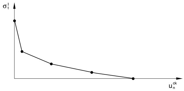# Implementation In Abaqus/Explicit this fracture energy cracking model can be invoked by specifying the postfailure stress as a tabular function of displacement across the crack, as illustrated in Figure 23.6.2–2. 

line

| u_n^ck | σ_t^I | | ------ | ----- | | 0 | 1.0 | | 1 | 0.5 | | 2 | 0.3 | | 3 | 0.2 | | 4 | 0.1 |

Figure 23.6.2–2 Postfailure stress-displacement curve. Alternatively, the Mode I fracture energy, $G _ { f } ^ { I }$ , can be specified directly as a material property; in this case, define the failure stress, $\sigma _ { t u } ^ { I } .$ as a tabular function of the associated Mode I fracture energy. This model assumes a linear loss of strength after cracking (Figure 23.6.2–3). The crack normal displacement at which complete loss of strength takes place is, therefore, $u _ { n 0 } = 2 G _ { f } ^ { I } / \sigma _ { t u } ^ { I }$ . Typical values of $G _ { f } ^ { I }$ range from 40 N/m (0.22 lb/in) for a typical construction concrete (with a compressive strength of approximately 20 MPa, 2850 lb/in2 ) to 120 N/m (0.67 lb/in) for a high-strength concrete (with a compressive strength of approximately 40 MPa, 5700 lb/in2 ). Input File Usage: Use the following option to specify the postfailure stress as a tabular function of displacement: $\mathrm { * B R I T T L E ~ C R A C K I N G } , \mathrm { T Y P E = D I S P L A C E M E N T }$