often provide accurate response in such cases, it is generally preferable to use structural elements (shells or beams) to model structural components. # Variable node elements Variable node elements (such as C3D27 and C3D15V) allow midface nodes to be introduced on any element face (on any rectangular face only for the triangular prism C3D15V). The choice is made by the nodes specified in the element definition. These elements are available only in Abaqus/Standard and can be used quite generally in any three-dimensional model. The C3D27 family of elements is frequently used as the ring of elements around a crack line. # Cylindrical elements Cylindrical elements (CCL9, CCL9H, CCL12, CCL12H, CCL18, CCL18H, CCL24, CCL24H, and CCL24RH) are available only in Abaqus/Standard for precise modeling of regions in a structure with circular geometry, such as a tire. The elements make use of trigonometric functions to interpolate displacements along the circumferential direction and use regular isoparametric interpolation in the radial or cross-sectional plane of the element. All the elements use three nodes along the circumferential direction and can span angles between 0 and 180°. Elements with both first-order and second-order interpolation in the cross-sectional plane are available. The geometry of the element is defined by specifying nodal coordinates in a global Cartesian system. The default nodal output is also provided in a global Cartesian system. Output of stress, strain, and other material point output quantities are done, by default, in a fixed local cylindrical system where direction 1 is the radial direction, direction 2 is the axial direction, and direction 3 is the circumferential direction. This default system is computed from the reference configuration of the element. An alternative local system can be defined (see “Orientations,” Section 2.2.5). In this case the output of stress, strain, and other material point quantities is done in the oriented system. The cylindrical elements can be used in the same mesh with regular elements. In particular, regular solid elements can be connected directly to the nodes on the cross-sectional plane of cylindrical elements. For example, any face of a C3D8 element can share nodes with the cross-sectional faces (faces 1 and 2; see “Cylindrical solid element library,” Section 28.1.5, for a description of the element faces) of a CCL12 element. Regular elements can also be connected along the circular edges of cylindrical elements by using a surface-based tie constraint (“Mesh tie constraints,” Section 35.3.1) provided that the cylindrical elements do not span a large segment. However, such usage may result in spurious oscillations in the solution near the tied surfaces and should be avoided when an accurate solution in this region is required. Compatible membrane elements (“Membrane elements,” Section 29.1.1) and surface elements with rebar (“Surface elements,” Section 32.7.1) are available for use with cylindrical solid elements. All elements with first-order interpolation in the cross-sectional plane use full integration for the deviatoric terms and reduced integration for the volumetric terms and, thus, have no hourglass modes and do not lock with almost incompressible materials. The hybrid elements with first-order and second-order interpolation in the cross-sectional plane use an independent interpolation for hydrostatic pressure. # Summary of recommendations for element usage The following recommendations apply to both Abaqus/Standard and Abaqus/Explicit: • Make all elements as “well shaped” as possible to improve convergence and accuracy. • If an automatic tetrahedral mesh generator is used, use the second-order elements C3D10 (in Abaqus/Standard) or C3D10M (in Abaqus/Explicit). Use the modified tetrahedral element C3D10M in Abaqus/Standard in analyses with large amounts of plastic deformation. • If possible, use hexahedral elements in three-dimensional analyses since they give the best results for the minimum cost. Abaqus/Standard users should also consider the following recommendations: • For linear and “smooth” nonlinear problems use reduced-integration, second-order elements if possible. • Use second-order, fully integrated elements close to stress concentrations to capture the severe gradients in these regions. However, avoid these elements in regions of finite strain if the material response is nearly incompressible. • Use first-order quadrilateral or hexahedral elements or the modified triangular and tetrahedral elements for problems involving large distortions. If the mesh distortion is severe, use reduced-integration, first-order elements. • If the problem involves bending and large distortions, use a fine mesh of first-order, reduced-integration elements. • Hybrid elements must be used if the material is fully incompressible (except when using plane stress elements). Hybrid elements should also be used in some cases with nearly incompressible materials. • Incompatible mode elements can give very accurate results in problems dominated by bending. # Naming convention The naming conventions for solid elements depend on the element dimensionality. 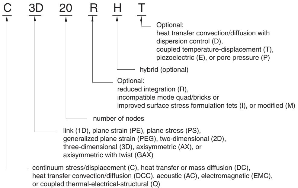# One-dimensional, two-dimensional, three-dimensional, and axisymmetric elements One-dimensional, two-dimensional, three-dimensional, and axisymmetric solid elements in Abaqus are named as shown below. For example, CAX4R is an axisymmetric continuum stress/displacement, 4-node, reduced-integration element; and CPS8RE is an 8-node, reduced-integration, plane stress piezoelectric element. The exception for this naming convention is C3D6 and C3D6T in Abaqus/Explicit, which are 6-node linear triangular prism, reduced integration elements. The pore pressure elements violate this naming convention slightly: the hybrid elements have the letter H after the letter P. For example, CPE8PH is an 8-node, hybrid, plane strain, pore pressure element. 

text_image

C 3D 20 R H T Optional: heat transfer convection/diffusion with dispersion control (D), coupled temperature-displacement (T), piezoelectric (E), or pore pressure (P) hybrid (optional) Optional: reduced integration (R), incompatible mode quad/bricks or improved surface stress formulation tets (I), or modified (M) number of nodes link (1D), plane strain (PE), plane stress (PS), generalized plane strain (PEG), two-dimensional (2D), three-dimensional (3D), axisymmetric (AX), or axisymmetric with twist (GAX) continuum stress/displacement (C), heat transfer or mass diffusion (DC), heat transfer convection/diffusion (DCC), acoustic (AC), electromagnetic (EMC), or coupled thermal-electrical-structural (Q)

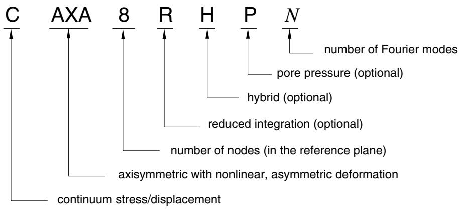
# Axisymmetric elements with nonlinear asymmetric deformation The axisymmetric solid elements with nonlinear asymmetric deformation in Abaqus/Standard are named as shown below. For example, CAXA4RH1 is a 4-node, reduced-integration, hybrid, axisymmetric element with nonlinear asymmetric deformation and one Fourier mode (see “Choosing the element’s dimensionality,” Section 27.1.2). 

text_image

C AXA 8 R H P N number of Fourier modes pore pressure (optional) hybrid (optional) reduced integration (optional) number of nodes (in the reference plane) axisymmetric with nonlinear, asymmetric deformation continuum stress/displacement

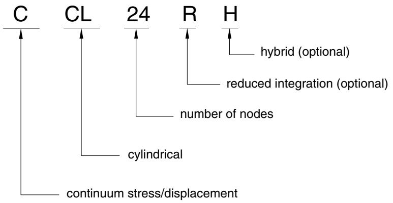
# Cylindrical elements The cylindrical elements in Abaqus/Standard are named as shown below. For example, CCL24RH is a 24-node, hybrid, reduced-integration cylindrical element. 

flowchart

```mermaid graph TD C --> A CL --> B 24 --> C R --> D H --> E C --> F CL --> G 24 --> H C --> H D --> H G --> H F --> H H --> H style C fill:#f9f,stroke:#333 style CL fill:#f9f,stroke:#333 style 24 fill:#f9f,stroke:#333 style R fill:#f9f,stroke:#333 style H fill:#f9f,stroke:#333 note right of C: "continuum stress/displacement" note right of C: "number of nodes" note right of D: "hybrid (optional)" note right of H: "reduced integration (optional)" ```

# Defining the element’s section properties A solid section definition is used to define the section properties of solid elements. In Abaqus/Standard solid elements can be composed of a single homogeneous material or can include several layers of different materials for the analysis of laminated composite solids. In Abaqus/Explicit solid elements can be composed only of a single homogeneous material. # Defining homogeneous solid elements You must associate a material definition (“Material data definition,” Section 21.1.2) with the solid section definition. In an Abaqus/Standard analysis spatially varying material behavior defined with one or more distributions (“Distribution definition,” Section 2.8.1) can be assigned to the solid section definition. In addition, you must associate the section definition with a region of your model. In Abaqus/Standard if any of the material behaviors assigned to the solid section definition (through the material definition) are defined with distributions, spatially varying material properties are applied to all elements associated with the solid section. Default material behaviors (as defined by the distributions) are applied to any element that is not specifically included in the associated distribution. Input File Usage: \*SOLID SECTION, MATERIAL=name, ELSET=name where the ELSET parameter refers to a set of solid elements. Abaqus/CAE Usage: Property module: Create Section: select Solid as the section Category and Homogeneous or Electromagnetic, Solid as the section Type: Material: name Assign→Section: select regions # Assigning an orientation definition You can associate a material orientation definition with solid elements (see “Orientations,” Section 2.2.5). A spatially varying local coordinate system defined with a distribution (“Distribution definition,” Section 2.8.1) can be assigned to the solid section definition. If the orientation definition assigned to the solid section definition is defined with distributions, spatially varying local coordinate systems are applied to all elements associated with the solid section. A default local coordinate system (as defined by the distributions) is applied to any element that is not specifically included in the associated distribution. Input File Usage: \*SOLID SECTION, ORIENTATION=name Abaqus/CAE Usage: Property module: Assign→Material Orientation # Defining the geometric attributes, if required For some element types additional geometric attributes are required, such as the cross-sectional area for one-dimensional elements or the thickness for two-dimensional plane elements. The attributes required for a particular element type are defined in the solid element libraries. These attributes are given as part of the solid section definition. # Defining composite solid elements in Abaqus/Standard The use of composite solids is limited to three-dimensional brick elements that have only displacement degrees of freedom (they are not available for coupled temperature-displacement elements, piezoelectric elements, pore pressure elements, and continuum cylindrical elements). Composite solid elements are primarily intended for modeling convenience. They usually do not provide a more accurate solution than composite shell elements. The thickness, the number of section points required for numerical integration through each layer (discussed below), and the material name and orientation associated with each layer are specified as part of the composite solid section definition. In Abaqus/Standard spatially varying orientation angles can be specified on a layer using distributions (“Distribution definition,” Section 2.8.1). The material layers can be stacked in any of the three isoparametric coordinates, parallel to opposite faces of the isoparametric master element as shown in Figure 28.1.1–1. The number of integration points within a layer at any given section point depends on the element type. Figure 28.1.1–1 shows the integration points for a fully integrated element.The element faces are defined by the order in which the nodes are specified when the element is defined. 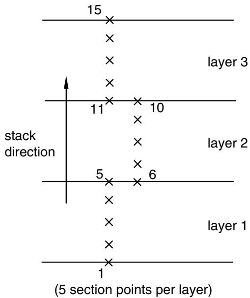The element matrices are obtained by numerical integration. Gauss quadrature is used in the plane of the lamina, and Simpson’s rule is used in the stacking direction. If one section point through the layer is used, it will be located in the middle of the layer thickness. The location of the section points in the plane of the lamina coincides with the location of the integration points. The number of section points required for the integration through the thickness of each layer is specified as part of the solid section definition; this number must be an odd number. The integration points for a fully integrated second-order composite element are shown in Figure 28.1.1–1, and the numbering of section points that are associated with an arbitrary integration point in a composite solid element is illustrated in Figure 28.1.1–2.  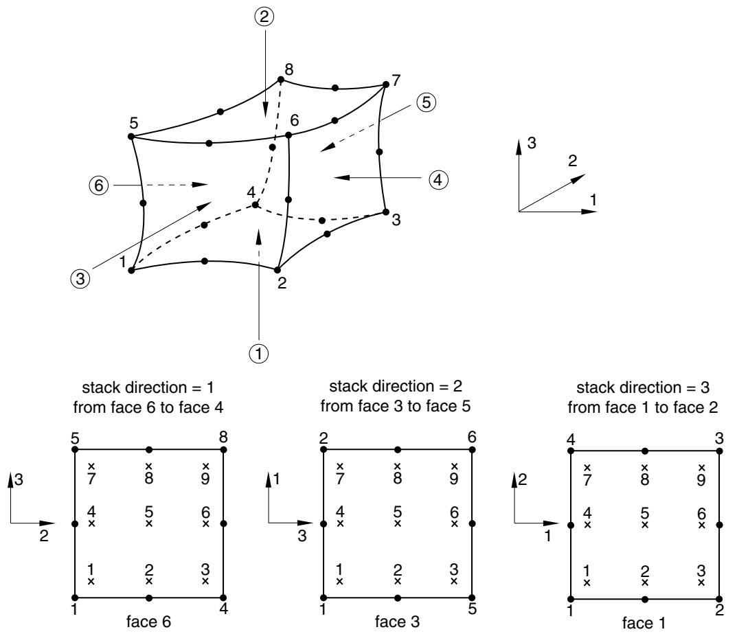Figure 28.1.1–1 Stacking direction and associated element faces and positions of element integration point output variables in the layer plane. 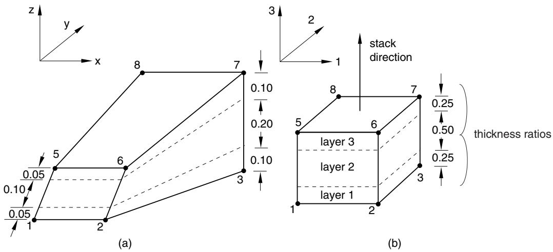The thickness of each layer may not be constant from integration point to integration point within an element since the element dimensions in the stack direction may vary. Therefore, it is defined indirectly by specifying the ratio between the thickness and the element length along the stack direction in the solid section definition, as shown in Figure 28.1.1–3. Using the ratios that are defined for all layers, actual thicknesses will be determined at each integration point such that their sum equals the element length in the stack direction. The thickness ratios for the layers need not reflect actual element or model dimensions. Unless your model is relatively simple, you will find it increasingly difficult to define your model using composite solid sections as you increase the number of layers and as you assign different sections to different regions. It can also be cumbersome to redefine the sections after you add new layers or remove or reposition existing layers. To manage a large number of layers in a typical composite model, you may 

scatter

| layer | stack direction | point count | |---------|-----------------|-------------| | layer 1 | 1 | 1 | | layer 1 | 5 | 5 | | layer 1 | 6 | 6 | | layer 2 | 11 | 11 | | layer 2 | 10 | 10 | | layer 3 | 15 | 15 |

Figure 28.1.1–2 Numbering of section points in a three-layered composite element. composite solid section with the material layers stacked in direction 3 

text_image

z y x 8 7 3 2 1 stack direction 5 6 3 0.10 0.20 0.10 0.05 0.10 0.05 (a) 8 7 5 6 layer 3 0.25 0.50 thickness ratios layer 2 layer 1 1 2 3 (b)

Figure 28.1.1–3 Lamina in (a) real space and (b) isoparametric space. want to use the composite layup functionality in Abaqus/CAE. For more information, see Chapter 23, “Composite layups,” of the Abaqus/CAE User’s Guide. For postprocessing composite solid elements appear in the output database (.odb) file with C1, C2, or C3 appended to the element type to represent the stacking direction of 1, 2, or 3, respectively.

Input File Usage:

*SOLID SECTION, COMPOSITE, STACK DIRECTION=1, 2, or 3, ELSET=name thickness, number of integration points, material name, orientation name

Abaqus/CAE Usage: Abaqus/CAE uses a composite layup or a composite solid section to define the layers of a composite solid. Use the following option for a composite layup: Property module: Create Composite Layup: select Solid as the Element Type: specify stacking direction, regions, thicknesses, number of integration points, materials, and orientations Use the following options for a composite solid section: Property module: Create Section: select Solid as the section Category and Composite as the section Type Assign→Material Orientation: select regions: Use Default Orientation or Other Method: Stacking Direction: Element direction 1, Element direction 2, Element direction 3, or From orientation Assign→Section: select regions # Output locations for composite solid elements You specify the location of the output variables in the plane of the lamina (layers) when you request output of element variables. For example, you can request values at the centroid of each layer. In addition, you specify the number of output points through the thickness of the layers by providing a list of the “section points.” The default section points for the output are the first and the last section point corresponding to the bottom and the top face, respectively (see Figure 28.1.1–2). See “Element output” in “Output to the data and results files,” Section 4.1.2, and “Element output” in “Output to the output database,” Section 4.1.3, for more information. # Modeling thick composites with solid elements in Abaqus/Standard While laminated composite solids are typically modeled using shell elements, the following cases require three-dimensional brick elements with one or multiple brick elements per layer: when transverse shear effects are predominant; when the normal stress cannot be ignored; and when accurate interlaminar stresses are required, such as near localized regions of complex loading or geometry. One case in which shell elements perform somewhat better than solid elements is in modeling the transverse shear stress through the thickness. The transverse shear stresses in solid elements usually do not vanish at the free surfaces of the structure and are usually discontinuous at layer interfaces. This deficiency may be present even if several elements are used in the discretization through the section thickness. Since the transverse shear stresses in thick shell elements are calculated by Abaqus on the basis of linear elasticity theory, such stresses are often better estimated by thick shell elements than by solid elements (see “Composite shells in cylindrical bending,” Section 1.1.3 of the Abaqus Benchmarks Guide). # Defining pressure loads on continuum elements The convention used for pressure loading on a continuum element is that positive pressure is directed into the element; that is, it pushes on the element. In large-strain analyses special consideration is necessary for plane stress elements that are pressure loaded on their edges; this issue is discussed in “Distributed loads,” Section 34.4.3. # Using solid elements in a rigid body All solid elements can be included in a rigid body definition. When solid elements are assigned to a rigid body, they are no longer deformable and their motion is governed by the motion of the rigid body reference node (see “Rigid body definition,” Section 2.4.1). Section properties for solid elements that are part of a rigid body must be defined to properly account for rigid body mass and rotary inertia. All associated material properties will be ignored except for the density. Element output is not available for solid elements assigned to a rigid body. # Automatic conversion of certain element types in Abaqus/Standard Element types C3D20 and C3D15 are converted automatically to the corresponding variable node element types C3D27 and C3D15V, respectively, if they have faces that are part of the slave surface in a node-to-surface contact pair (see “Adjusting contact controls in Abaqus/Standard,” Section 36.3.6). # Special considerations for various element types in Abaqus/Standard The following considerations should be acknowledged in the context of the stress/displacement, coupled temperature-displacement, and heat transfer elements in Abaqus/Standard. # Interpolation of temperature and field variables in stress/displacement elements The value of temperatures at the integration points used to compute the thermal stresses depends on whether first-order or second-order elements are used. An average temperature is used at the integration points in (compatible) linear elements so that the thermal strain is constant throughout the element; in the case of elements with incompatible modes the temperatures are interpolated linearly. An approximate linearly varying temperature distribution is used in higher-order elements with full integration. Higherorder reduced-integration elements pose no special problems since the temperatures are interpolated linearly. Field variables in a given stress/displacement element are interpolated using the same scheme used to interpolate temperatures. # Interpolation in coupled temperature-displacement elements Coupled temperature-displacement elements use either linear or parabolic interpolation for the geometry and displacements. Temperature is interpolated linearly, but certain rules can apply to the temperature and field variable evaluation at the Gauss points, as discussed below. The elements that use linear interpolation for displacements and temperatures have temperatures at all nodes. The thermal strain is taken as constant throughout the element because it is desirable to have the same interpolation for thermal strains as for total strains so as to avoid spurious hydrostatic stresses. Separate integration schemes are used for the internal energy storage, heat conduction, and plastic dissipation (coupling contribution) terms for the first-order elements. The internal energy storage term is integrated at the nodes, which yields a lumped internal energy matrix and, thereby, improves the accuracy for problems with latent heat effects. In fully integrated elements both the heat conduction and plastic dissipation terms are integrated at the Gauss points. While the plastic dissipation term is integrated at each Gauss point, the heat generated by the mechanical deformation at a Gauss point is applied at the nearest node. The temperature at a Gauss point is assumed to be the temperature of its nearest node to be consistent with the temperature treatment throughout the formulation. In reducedintegration elements the plastic dissipation term is obtained at the centroid and the heat generated by the mechanical deformation is applied as a weighted average at each node. The temperature at the centroid of reduced-integration elements is a weighted average of the nodal temperatures to be consistent with the temperature treatment throughout the formulation. The elements that use parabolic interpolation for displacements and linear interpolation for temperatures have displacement degrees of freedom at all of the nodes, but temperature degrees of freedom exist only at the corner nodes. The temperatures are interpolated linearly so that the thermal strains have the same interpolation as the total strains. Temperatures at the midside nodes are calculated by linear interpolation from the corner nodes for output purposes only. In contrast to the linear coupled elements, all terms in the governing equations are integrated using a conventional Gauss scheme. For these elements the stiffness matrix can be generated using either full integration (3 Gauss points in each parametric direction) or reduced integration (2 Gauss points in each parametric direction). The same integration scheme is always used for the specific heat and conductivity matrices as for the stiffness matrix; however, because of the lower-order interpolation for temperature, this implies that we always use a full integration scheme for the heat transfer matrices, even when the stiffness integration is reduced. Reduced integration uses a lower-order integration to form the element stiffness: the mass matrix and distributed loadings are still integrated exactly. Reduced integration usually provides more accurate results (providing that the elements are not distorted) and significantly reduces running time, especially in three dimensions. Reduced integration for the quadratic displacement elements is recommended in all cases except when very sharp strain gradients are expected (such as in finite-strain metal forming applications); these elements are considered to be the most cost-effective elements of this class. The value of field variables at the integration points depends on whether first-order or second-order coupled temperature-displacement elements are used. An average field variable is used at the integration points in linear elements. An approximate linearly varying field variable distribution is used in higherorder elements with full integration. Higher-order reduced-integration elements pose no special problems since the field variables are interpolated linearly. Modified triangle and tetrahedron elements use a special consistent interpolation scheme for displacement and temperature. Displacement and temperature degrees of freedom are active at all user-defined nodes.