# 29.3.2 CHOOSING A BEAM CROSS-SECTION Products: Abaqus/Standard Abaqus/Explicit Abaqus/CAE # References • “Beam modeling: overview,” Section 29.3.1 • “Beam cross-section library,” Section 29.3.9 • “Meshed beam cross-sections,” Section 10.6.1 • “Defining profiles,” Section 12.2.2 of the Abaqus/CAE User’s Guide # Overview The choice of cross-section is determined by the geometry of the cross-section and its behavior. A beam’s cross-section: • can be solid or thin-walled; • if thin-walled, can be open or closed; and • can be defined by choosing from the Abaqus cross-section library; by specifying geometric quantities such as area, moments of inertia, and torsional constant; or by using a mesh of special two-dimensional elements, for which geometric quantities are calculated numerically. You must consider whether the section should be treated as a solid cross-section or as a thin-walled cross-section. This choice determines the basis upon which Abaqus computes the axial and shear strains at each point in the section. # Solid cross-sections For solid sections under bending, plane (beam) sections remain plane. Under torsional loading any noncircular beam section will warp: the beam section will not remain planar. However, for solid sections the warping of the section is small enough so that the axial strain due to warping of the section can be neglected and St. Venant warping theory can be used to construct a single component of shear strain at each integration point in the section. This is done automatically for the rectangular and trapezoidal sections in the beam section library. The St. Venant warping functions are used to define the shear strain even when the response in the section is no longer purely elastic. This limits the accuracy of the modeling for cases involving noncircular solid beam sections subjected to torsional loadings that cause large amounts of inelastic deformation. When using a meshed beam profile, two shear strain components are available for output in the user-specified material system. The thick pipe section is treated as a solid cross-section. # Nonsolid (“thin-walled”) cross-sections In Abaqus nonsolid sections are treated as “thin-walled” sections; that is, in the plane of the section, the thickness of a branch of the section is assumed to be small compared to its length. Thin-walled beam theory determines the shear in the wall of the section depending on whether the section is closed or open. # Closed sections A closed section is a nonsolid section whose branches form closed loops. Closed sections offer significant resistance to torsion and do not warp significantly. Abaqus ignores warping effects for closed sections. In Abaqus predefined beam sections can model only one closed loop. Sections with multiple loops must be modeled with a meshed beam section (see “Meshed cross-sections”) or with shells. For sufficiently small thickness of the section walls, the variation of shear stress across the thickness is negligible; the formulation of the closed sections available in Abaqus is based on this assumption. # Open sections An open section is a nonsolid section with branches that do not form closed loops, such as an I-section or a U-section. In such sections the shear stress is assumed to vary linearly over the wall thickness and to vanish at the center of the wall. Open sections can warp significantly and generally require the use of open-section warping theory (available with beam element types BxxOS in Abaqus/Standard) with suitable warping constraints (applied to degree of freedom 7) at supports or joints. Such warping constraints may significantly increase the torsional stiffness of the beam. Open, thin-walled sections whose branches are straight lines that meet at a single point (such as the L-section in the Abaqus beam element section library, T-sections, or X-sections) do not warp; therefore, warping constraints have no effect. Such sections always have very little torsional stiffness. If an open section is used with a regular beam element type (not BxxOS), the open section is assumed to be free to warp and the axial strain due to warping is neglected. Consequently, the section will have very little torsional stiffness. # Section property calculations Thin-walled assumptions are used when calculating nonsolid section properties. Properties for sections comprised of intersecting straight segments (arbitrary, box, hexagonal, I-, and L-sections) also include an approximation of the intersection geometry. # Available beam cross-sections You can specify any of the following types of beam cross-sections: an Abaqus library cross-section, a generalized cross-section for which you specify the geometric quantities directly, or a meshed crosssection. # The Abaqus beam cross-section library The Abaqus beam cross-section library contains solid sections (circular, rectangular, and trapezoidal), closed thin-walled sections (box, hexagonal, and pipe), open thin-walled sections (I-shaped, T-shaped, or L-shaped), and a thick-walled pipe section. Abaqus also provides an arbitrary thin-walled section definition; Abaqus will treat this section type as a closed or open section, depending on how the section is defined. Trapezoidal, I, and arbitrary library sections allow you to define the location of the origin of the local coordinate system. Other section types—such as rectangular, circular, L, or pipe—have preset origins. Input File Usage: Use the following option to define a beam section integrated during the analysis: \*BEAM SECTION, SECTION=name where name can be ARBITRARY, BOX, CIRC, HEX, I, L, PIPE, RECT, THICK PIPE, or TRAPEZOID. A T-section is defined by specifying geometric data for only one flange of an I-section. Use the following option to define a general beam section: \*BEAM GENERAL SECTION, SECTION=name where name can be ARBITRARY, BOX, CIRC, HEX, I, L, PIPE, RECT, or TRAPEZOID. A T-section is defined by specifying geometric data for only one flange of an I-section. Abaqus/CAE Usage: Property module: Create Profile: choose Box, Pipe, Circular, Rectangular, Hexagonal, Trapezoidal, I, L, T, or Arbitrary # Generalized cross-sections Abaqus also allows you to specify “generalized” cross-sections by specifying the geometric quantities necessary to define the section. Such generalized sections can be used only with linear material behavior although the section response can be linear or nonlinear. Input File Usage: Use the following option to define a linear generalized cross-section: \*BEAM GENERAL SECTION, SECTION=GENERAL Use the following option to define a nonlinear generalized cross-section: \*BEAM GENERAL SECTION, SECTION=NONLINEAR GENERAL Abaqus/CAE Usage: Property module: Create Profile: choose Generalized Nonlinear generalized cross-sections are not supported in Abaqus/CAE. # Meshed cross-sections Abaqus allows you to mesh an arbitrarily shaped solid cross-section by using warping elements (see “Warping elements,” Section 28.4.1) in a two-dimensional analysis to generate beam cross-section properties that can be used in a subsequent two- or three-dimensional beam analysis. Such sections permit only linear, elastic material behavior. Therefore, a meshed cross-section can be used only with a general beam section definition; for details, see “Meshed beam cross-sections,” Section 10.6.1. Input File Usage: \*BEAM GENERAL SECTION, SECTION=MESHED Abaqus/CAE Usage: Meshed cross-sections are not supported in Abaqus/CAE. # 29.3.3 CHOOSING A BEAM ELEMENT Products: Abaqus/Standard Abaqus/Explicit Abaqus/CAE # References • “Beam modeling: overview,” Section 29.3.1 • “Beam element library,” Section 29.3.8 • \*TRANSVERSE SHEAR STIFFNESS • “Creating beam sections,” Section 12.13.11 of the Abaqus/CAE User’s Guide, in the HTML version of this guide # Overview Abaqus offers a wide range of beam elements, including “Euler-Bernoulli”-type beams and “Timoshenko”-type beams with solid, thin-walled closed and thin-walled open sections. The Abaqus/Standard beam element library includes: • Euler-Bernoulli (slender) beams in a plane and in space; • Timoshenko (shear flexible) beams in a plane and in space; • linear, quadratic, and cubic interpolation formulations; • warping (open section) beams; • pipe elements; and • hybrid formulation beams, typically used for very stiff beams that rotate significantly (applications in robotics or in very flexible structures such as offshore pipelines). The Abaqus/Explicit beam element library includes: • Timoshenko (shear flexible) beams in a plane and in space; • linear and quadratic interpolation formulations; and • linear pipe elements. # Naming convention Beam elements in Abaqus are named as follows: 

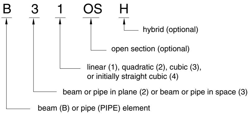
text_image

B 3 1 OS H hybrid (optional) open section (optional) linear (1), quadratic (2), cubic (3), or initially straight cubic (4) beam or pipe in plane (2) or beam or pipe in space (3) beam (B) or pipe (PIPE) element

For example, B21H is a planar beam that uses linear interpolation and a hybrid formulation. # Euler-Bernoulli (slender) beams Euler-Bernoulli beams (B23, B23H, B33, and B33H) are available only in Abaqus/Standard. These elements do not allow for transverse shear deformation; plane sections initially normal to the beam’s axis remain plane (if there is no warping) and normal to the beam axis. They should be used only to model slender beams: the beam’s cross-sectional dimensions should be small compared to typical distances along its axis (such as the distance between support points or the wavelength of the highest mode that participates in a dynamic response). For beams made of uniform material, typical dimensions in the cross-section should be less than about 1/15 of typical axial distances for transverse shear flexibility to be negligible. (The ratio of cross-section dimension to typical axial distance is called the slenderness ratio.) Load stiffness for pressure loads is not included for these elements. # Interpolation The Euler-Bernoulli beam elements use cubic interpolation functions, which makes them reasonably accurate for cases involving distributed loading along the beam. Therefore, they are well suited for dynamic vibration studies, where the d’Alembert (inertia) forces provide such distributed loading. The cubic beam elements are written for small-strain, large-rotation analysis. They may not be appropriate for torsional stability problems due to the approximations in the underlying formulation and cannot be used in analyses involving very large rotations (of the order 180°); quadratic or linear beam elements should be used instead. # Mass formulation The Euler-Bernoulli beam elements use a consistent mass formulation. Rotary inertia for twist around the beam axis is the same as for Timoshenko beams. For details, see “Mass and inertia for Timoshenko beams,” Section 3.5.5 of the Abaqus Theory Guide. Any additional inertia defined for these elements (see “Adding inertia to the beam section behavior for Timoshenko beams” in “Beam section behavior,” Section 29.3.5) is ignored. Timoshenko beams (B21, B22, B31, B31OS, B32, B32OS, PIPE21, PIPE22, PIPE31, PIPE32, and their “hybrid” equivalents) allow for transverse shear deformation. They can be used for thick (“stout”) as well as slender beams. For beams made from uniform material, shear flexible beam theory can provide useful results for cross-sectional dimensions up to 1/8 of typical axial distances or the wavelength of the highest natural mode that contributes significantly to the response. Beyond this ratio the approximations that allow the member’s behavior to be described solely as a function of axial position no longer provide adequate accuracy. Abaqus assumes that the transverse shear behavior of Timoshenko beams is linear elastic with a fixed modulus and, thus, independent of the response of the beam section to axial stretch and bending. For most beam sections Abaqus will calculate the transverse shear stiffness values required in the element formulation. You can override these default values as described below in “Defining the transverse shear stiffness and the slenderness compensation factor.” The default shear stiffness values are not calculated in some cases if estimates of shear moduli are unavailable during the preprocessing stage of input; for example, when the material behavior is defined by user subroutine UMAT, UHYPEL, UHYPER, or VUMAT. In such cases you must define the transverse shear stiffnesses as described below. The Timoshenko beams can be subjected to large axial strains. The axial strains due to torsion are assumed to be small. In combined axial-torsion loading, torsional shear strains are calculated accurately only when the axial strain is not large. # Transverse shear stiffness definition The effective transverse shear stiffness of the section of a shear flexible beam is defined in Abaqus as $$ \bar {K} _ {\alpha 3} = f _ {p} ^ {\alpha} K _ {\alpha 3}, $$ where $\bar { K } _ { \alpha 3 }$ is the section shear stiffness in the -direction; $f _ { p } ^ { \alpha }$ is a dimensionless factor used to prevent the shear stiffness from becoming too large in slender beam elements; $K _ { \alpha 3 }$ is the actual shear stiffness of the section; and $\alpha = 1 , 2$ are the local directions of the cross-section. The $K _ { \alpha 3 }$ have units of force. The dimensionless factors $f _ { p } ^ { \alpha }$ are always included in the calculation of transverse shear stiffness and are defined as $$ f _ {p} ^ {\alpha} = 1 / (1 + \xi * S C F \frac {l ^ {2} A}{1 2 I _ {\alpha \alpha}}), $$ where l is the length of the element, A is the cross-sectional area, $I _ { \alpha \alpha }$ is the inertia in the -direction, $S C F$ is the slenderness compensation factor (with a default value of 0.25), and $\xi$ is a constant of value 1.0 for first-order elements and $1 0 ^ { - 4 }$ for second-order elements. For meshed cross-sections the above expressions change to $$ \bar {K} _ {\alpha \beta} ^ {t s} = f _ {p} K _ {\alpha \beta} ^ {t s}, $$ $$ f _ {p} = 1 / (1 + \xi * S C F \frac {l ^ {2} (E A)}{1 2 (E I) _ {a v}}), $$ $$ (E I) _ {a v} = 1 / 3 ((E I) _ {1 1} + (E I) _ {2 2} + (E I) _ {1 2}). $$ You can define the $K _ { \alpha 3 }$ or $K _ { \alpha \beta } ^ { t s }$ as described below. If you do not specify them, they are defined by $$ K _ {\alpha 3} = k G A, $$ or $$ K _ {\alpha \beta} ^ {t s} = k (G A) _ {\alpha \beta}, $$ where G is the elastic shear modulus or moduli and A is the cross-sectional area of the beam section. Temperature and field variable dependencies of G are not taken into account when calculating $K _ { \alpha 3 }$ and $K _ { \alpha \beta } ^ { t s }$ . The shear factor k (Cowper, 1966) is defined as:

Section type	Shear factor, k
Arbitrary	1.0
Box	0.44
Circular	0.89
Elbow	0.85
Generalized	1.0
Hexagonal	0.53
I (and T)	0.44
L	1.0
Meshed	1.0
Nonlinear generalized	1.0
Pipe	0.53
Rectangular	0.85
Thick pipe	0.53–0.89
Trapezoidal	0.822

When a beam section definition integrated during the analysis is used (see “Using a beam section integrated during the analysis to define the section behavior,” Section 29.3.6), G is calculated from the elastic material definition used with the section. When a general beam section definition is used (see “Using a general beam section to define the section behavior,” Section 29.3.7), you provide G as part of the beam section data. # Defining the transverse shear stiffness and the slenderness compensation factor You can define the transverse shear stiffness for beam sections integrated during the analysis and general beam sections. In the case of two-dimensional beams, you can input a single value of transverse shear stiffness, namely $K _ { 2 3 }$ . If either value of $K _ { \alpha 3 }$ is omitted or given as zero, the nonzero value will be used for both. You can also define the slenderness compensation factor. The default value for the slenderness compensation factor is 0.25. If a slenderness compensation factor value is provided, you must also provide the values of the shear stiffness $K _ { \alpha 3 }$ . In the case of first-order elements, you may define the slenderness compensation factor by including the label SCF. Abaqus will then use a slenderness compensation factor of $\begin{array} { r } { \bar { S } C F = \frac { k G A } { E A } } \end{array}$ , and any values of $K _ { \alpha 3 }$ that you specify are ignored. Instead, the $K _ { \alpha 3 }$ values are calculated from the elastic material definition. The transverse shear stiffness is not relevant to Euler-Bernoulli beam elements for which the transverse shear constraints are satisfied exactly. Input File Usage: Use both of the following options to define the transverse shear stiffness for beam sections integrated during the analysis: \*BEAM SECTION \*TRANSVERSE SHEAR STIFFNESS Use both of the following options to define the transverse shear stiffness for general beam sections: \*BEAM GENERAL SECTION \*TRANSVERSE SHEAR STIFFNESS Abaqus/CAE Usage: To define transverse shear stiffness for beam sections integrated during the analysis: Property module: beam section editor: Section integration: During analysis: Stiffness: toggle on Specify transverse shear To define transverse shear stiffness for general beam sections: Property module: beam section editor: Section integration: Before analysis: Stiffness, toggle on Specify transverse shear # Interpolation Abaqus provides finite axial strain, shear flexible beams with linear and quadratic interpolations. Their formulation is described in “Beam element formulation,” Section 3.5.2 of the Abaqus Theory Guide. Element types B21, B31, B31OS, PIPE21, PIPE31, and their hybrid equivalents use linear interpolation. These elements are well suited for cases involving contact, such as the laying of a pipeline in a trench or on the seabed or the contact between a drill string and a well hole, and for dynamic versions of similar problems (impact). Element types B22, B32, B32OS, PIPE22, PIPE32, and their hybrid equivalents use quadratic interpolation. # Mass formulation The linear Timoshenko beam elements use a lumped mass formulation by default. The quadratic Timoshenko beam elements in Abaqus/Standard use a consistent mass formulation, except in dynamic procedures in which a lumped mass formulation with a 1/6, 2/3, 1/6 distribution is used. For details, see “Mass and inertia for Timoshenko beams,” Section 3.5.5 of the Abaqus Theory Guide. The quadratic Timoshenko beam elements in Abaqus/Explicit use a lumped mass formulation with a 1/6, 2/3, 1/6 distribution. Using a consistent mass matrix in Abaqus/Standard Alternatively, in Abaqus/Standard you can use the McCalley-Archer consistent mass matrix based on the cubic interpolation of deflections and quadratic interpolation of rotations. Input File Usage: Use the following option for linear Timoshenko beam elements with beam sections integrated during the analysis: \*BEAM SECTION, LUMPED=NO Use the following option for linear Timoshenko beam elements with general beam sections: \*BEAM GENERAL SECTION, LUMPED=NO Abaqus/CAE Usage: Use the following option for linear Timoshenko beam elements with beam sections integrated during the analysis: Property module: beam section editor: Section integration: During analysis: Stiffness tabbed page: toggle on Use consistent mass matrix formulation Use the following option for linear Timoshenko beam elements with general beam sections: Property module: beam section editor: Section integration: Before analysis: Stiffness tabbed page: toggle on Use consistent mass matrix formulation # Rotary inertia treatment and additional beam inertia By default, the exact (anisotropic with displacement-rotation coupling) rotary inertia is used for Timoshenko beams. Optionally, an uncoupled isotropic approximation to the rotary inertia can be used. See “Rotary inertia for Timoshenko beams” in “Beam section behavior,” Section 29.3.5, for further details. The exception to this rule is the static procedure with automatic stabilization (see “Static stress analysis,” Section 6.2.2), where the mass matrix for Timoshenko beams is always calculated assuming isotropic rotary inertia, regardless of the type of rotary inertia specified for the beam section definition (see “Rotary inertia for Timoshenko beams” in “Beam section behavior,” Section 29.3.5).