# CVJOINT Connection type CVJOINT joins the position of two nodes and provides a constant velocity constraint between their rotational degrees of freedom. Connection type CVJOINT cannot be used in two-dimensional or axisymmetric analysis. 

text_image

Diagram illustrating magnetic field vectors and rotational motion with labeled vectors and angular relationships

Figure 31.1.5–10 Connection type CVJOINT. # Description Connection type CVJOINT imposes kinematic constraints and uses local orientation definitions equivalent to combining connection types JOIN and CONSTANT VELOCITY. # Summary

CVJOINT
Basic, assembled, or complex:	Assembled
Kinematic constraints:	JOIN + CONSTANT VELOCITY
Constraint force and moment output:	$f_1, f_2, f_3, m_2$
Available components:	None
Kinetic force and moment output:	None
Orientation at a:	Required
Orientation at b:	Optional
Connector stops:	None
Constitutive reference lengths and angles:	None
Predefined friction parameters:	None
Contact force for predefined friction:	None

# CYLINDRICAL Connection type CYLINDRICAL provides a slot connection between two nodes and a revolute constraint where the free rotation is about the line of the slot. It cannot be used in two-dimensional or axisymmetric analysis. 

text_image

e₂ᵃ e₂ᵇ e₁ᵇ a e₁ᵃ b e₃ᵃ e₃ᵇ u₁ ur₁

Figure 31.1.5–11 Connection type CYLINDRICAL. # Description Connection type CYLINDRICAL imposes kinematic constraints and uses local orientation definitions equivalent to combining connection types SLOT and REVOLUTE. The connector constraint forces and moments reported as connector output depend strongly on the order and the location of the nodes in the connector (see “Connector behavior,” Section 31.2.1). Since the kinematic constraints are enforced at node b (the second node of the connector element), the reported forces and moments are the constraint forces and moments applied at node b to enforce the CYLINDRICAL constraint. Thus, in most cases the connector output associated with a CYLINDRICAL connection is best interpreted when node b is located at the center of the device enforcing the constraint. This choice is essential when moment-based friction is modeled in the connector since the contact forces are derived on the connector forces and moments, as illustrated below. Proper enforcement of the kinematic constraints is independent of the order or location of the nodes. # Friction Predefined Coulomb-like friction in the CYLINDRICAL connection defines the friction force (CSFC) along the instantaneous slip direction on the two contacting cylindrical surfaces (the pin and the sleeve) illustrated above. The table below summarizes the parameters that are used to specify predefined friction in this connection type as discussed in detail next. The frictional effect is formally written as $$ \Phi = \mathrm{P} (\mathbf {f}) - \mu \mathrm{F} _ {\mathrm{N}} \leq 0, $$ where the potential $\mathrm { P } ( \mathbf { f } )$ represents the magnitude of the frictional tangential tractions in the connector in a direction tangent to the cylindrical surface on which contact occurs, $\mathrm { F _ { N } }$ is the friction-producing normal force on the same cylindrical surface, and $\mu$ is the friction coefficient. Frictional stick occurs if $\Phi < 0 ;$ and sliding occurs if $\Phi = 0$ , in which case the friction force is $\mu \mathrm { F _ { N } }$ . The normal force $\mathrm { F _ { N } }$ is the sum of a magnitude measure of friction-producing connector forces, $\mathrm { F } _ { \mathrm { C } } = g ( \mathbf { f } )$ , and a self-equilibrated internal contact force (such as from a press-fit assembly), $\mathrm { F _ { C } ^ { \mathrm { i n t } } }$ : $$ \mathrm {F_ {N}} = | \mathrm {F_ {C}} + \mathrm {F_ {C} ^ {int}} | = | g (\mathbf {f}) + \mathrm {F_ {C} ^ {int}} |. $$ The magnitude measure of friction-producing connector contact force, $\mathrm { F _ { C } , }$ is defined by summing the following two contributions: • a radial force contribution, $F _ { r }$ (the magnitude of the constraint forces enforcing the SLOT constraint): $$ F _ {r} = \sqrt {f _ {2} ^ {2} + f _ {3} ^ {2}}, \mathrm{and} $$ • a force contribution from “bending,” $F _ { b e n d : }$ , obtained by scaling the bending moment, $M _ { b e n d }$ (the magnitude of the constraint moments enforcing the REVOLUTE constraint), by a length factor, as follows: $$ M _ {b e n d} = \sqrt {m _ {2} ^ {2} + m _ {3} ^ {2}}, $$ $$ F _ {b e n d} = 2 \frac {M _ {b e n d}}{L}, $$ where L represents a characteristic overlapping length between the shaft and the outer sleeve in the 1-direction. If L is $0 . 0 , M _ { b e n d }$ is ignored. Thus, $$ \mathrm {F_ {C}} = g (\mathbf {f}) = F _ {r} + F _ {b e n d} = \sqrt {f _ {2} ^ {2} + f _ {3} ^ {2}} + \sqrt {(\beta m _ {2}) ^ {2} + (\beta m _ {3}) ^ {2}}, $$ where $\begin{array} { r } { \beta = \frac { 2 } { L } } \end{array}$ The magnitude of the frictional tangential moment, $\mathrm { P } ( \mathbf { f } )$ is computed using $$ \mathrm{P} (\mathbf {f}) = \sqrt {f _ {1} ^ {2} + (\frac {m _ {1}}{R}) ^ {2}}, $$ where R is an effective radius of the shaft cross-section in the local 2–3 plane. The potential represents the magnitude of connector tangential tractions on the cylindrical contact surface due to simultaneous translation and rotation. The instantaneous slip direction is a result of combined motion in these directions. Summary

CYLINDRICAL
Basic, assembled, or complex:	Assembled
Kinematic constraints:	SLOT + REVOLUTE
Constraint force and moment output:	$f_{2}, f_{3}, m_{2}, m_{3}$
Available components:	$u_{1}, ur_{1}$
Kinetic force and moment output:	$f_{1}, m_{1}$
Orientation at a:	Required
Orientation at b:	Optional
Connector stops:	$l_{1}^{min} \leq l \leq l_{1}^{max}$ $\theta_{1}^{min} \leq \alpha \leq \theta_{1}^{max}$
Constitutive reference lengths and angles:	$l_{1}^{ref}, \theta_{1}^{ref}$
Predefined friction parameters:	Required: R; optional: L, $F_{C}^{int}$
Contact force for predefined friction:	$F_{C}$

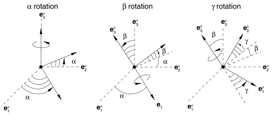
# EULER Connection type EULER provides a rotational connection between two nodes where the total relative rotation between the nodes is parameterized by Euler angles. An Euler-angle parameterization of finite rotations is also called a 3–1–3 or precession-nutation-spin parameterization. Connection type EULER cannot be used in two-dimensional or axisymmetric analysis.  Figure 31.1.5–12 Connection type EULER. # Description The EULER connection does not impose kinematic constraints. An EULER connection is a finite rotation connection where the local directions at node b are parameterized in terms of Euler angles relative to the local directions at node a. Local directions $\{ \mathbf { e } _ { 1 } ^ { b } , \mathbf { e } _ { 2 } ^ { b } , \mathbf { e } _ { 3 } ^ { b } \}$ are positioned relative to $\{ { \bf e } _ { 1 } ^ { a } , { \bf e } _ { 2 } ^ { a } , { \bf e } _ { 3 } ^ { a } \}$ by three successive finite rotations $\alpha , \beta ,$ , and $\gamma$ as follows: 1. Rotate by radians about axis ${ \bf e } _ { 3 } ^ { a }$ ; 2. Rotate by $\beta$ radians about the intermediate 1-axis, $\mathbf { e } _ { 1 } = \mathrm { c o s } \alpha \mathbf { e } _ { 1 } ^ { a } + \mathrm { s i n } \alpha \mathbf { e } _ { 2 } ^ { a } ;$ ; 3. Rotate by $\gamma$ radians about axis $\mathbf { e } _ { 3 } ^ { b }$ . The Euler angles are determined by the local directions as $$ \alpha = - \tan^ {- 1} \left(\frac {\mathbf {e} _ {1} ^ {a} \cdot \mathbf {e} _ {3} ^ {b}}{\mathbf {e} _ {2} ^ {a} \cdot \mathbf {e} _ {3} ^ {b}}\right) + i \pi ; $$ $$ \beta = \cos^ {- 1} \left(\mathbf {e} _ {3} ^ {a} \cdot \mathbf {e} _ {3} ^ {b}\right) + j \pi ; $$ $$ \gamma = \tan^ {- 1} \left(\frac {\mathbf {e} _ {3} ^ {a} \cdot \mathbf {e} _ {1} ^ {b}}{\mathbf {e} _ {3} ^ {a} \cdot \mathbf {e} _ {2} ^ {b}}\right) + k \pi . $$ Here $i , j ,$ and $\pmb { k }$ are integers that account for rotations with magnitudes greater than $\pi .$ . Initially, the intermediate rotation angle $\beta$ is chosen in the interval $0 \leq \beta \leq \pi$ . If the intermediate rotation is an even multiple of $\pi , \beta = 2 m \pi$ , where $m = 0 , \pm 1 , \pm 2 , . . .$ , the other two Euler angles become non-unique. In this case $$ \alpha + \gamma = \tan^ {- 1} \left(\frac {\mathbf {e} _ {2} ^ {a} \cdot \mathbf {e} _ {1} ^ {b}}{\mathbf {e} _ {1} ^ {a} \cdot \mathbf {e} _ {1} ^ {b}}\right) + n \pi . $$ Similarly, if the intermediate rotation is an odd multiple of $\pi , \beta = ( 2 m + 1 ) \pi$ , where $m = 0 , \pm 1 , \pm 2 , . . . _ $ the other two Euler angles become nonunique as well. In this case $$ \alpha - \gamma = \tan^ {- 1} \left(\frac {\mathbf {e} _ {2} ^ {a} \cdot \mathbf {e} _ {1} ^ {b}}{\mathbf {e} _ {1} ^ {a} \cdot \mathbf {e} _ {1} ^ {b}}\right) + n \pi . $$ In both of these cases a singularity results in the rotation parameterization when the ${ \bf e } _ { 3 } ^ { a }$ and $\mathbf { e } _ { 3 } ^ { b }$ axes align. The EULER connection should be used in such a way that these axes do not align throughout the computation. For a singularity-free condition Abaqus will choose $\alpha$ and $\gamma$ such that a smooth parameterization results for the above values of the intermediate angle $\beta .$ The available components of relative motion in the EULER connection are the changes in the Euler angles that position the local directions at node b relative to the local directions at node a. Therefore, $$ u r _ {1} = \alpha - \alpha_ {0}; \quad u r _ {2} = \beta - \beta_ {0}; \quad \text {and} \quad u r _ {3} = \gamma - \gamma_ {0}; $$ where $\alpha _ { 0 } , \beta _ { 0 }$ , and $\gamma _ { 0 }$ are the initial Euler angles. The connector constitutive rotations are $$ u r _ {1} ^ {m a t} = \alpha - \theta_ {1} ^ {r e f}; \quad u r _ {2} ^ {m a t} = \beta - \theta_ {2} ^ {r e f}; \quad \text {and} \quad u r _ {3} ^ {m a t} = \gamma - \theta_ {3} ^ {r e f}. $$ The kinetic moment in a EULER connection is determined from the three component relationships: $$ \mathbf {m} _ {E u l e r} = m _ {1} \mathbf {e} _ {3} ^ {a} + m _ {2} \bigl (\cos \alpha \mathbf {e} _ {1} ^ {a} + \sin \alpha \mathbf {e} _ {2} ^ {a} \bigr) + m _ {3} \mathbf {e} _ {3} ^ {b}. $$ Summary # EULER

Basic, assembled, or complex:	Basic
Kinematic constraints:	None
Constraint moment output:	None
Available components:	$ur_{1}, ur_{2}, ur_{3}$

EULER

Kinetic moment output:	$m_{1}, m_{2}, m_{3}$
Orientation at a:	Required
Orientation at b:	Optional
Connector stops:	$\theta_{1}^{min} \leq \alpha \leq \theta_{1}^{max}$ , $\theta_{2}^{min} \leq \beta \leq \theta_{2}^{max}$ , $\theta_{3}^{min} \leq \gamma \leq \theta_{3}^{max}$
Constitutive reference angles:	$\theta_{1}^{ref}, \theta_{2}^{ref}, \theta_{3}^{ref}$
Predefined friction parameters:	None
Contact force for predefined friction:	None

# FLEXION-TORSION Connection type FLEXION-TORSION provides a rotational connection between two nodes. It models the bending and twisting of a cylindrical coupling between two shafts. In this case the response to twist rotations about the shafts may differ from the response to bending of the shafts. Connection type FLEXION-TORSION cannot be used in two-dimensional or axisymmetric analysis. The flexural part of the connection resists angular misalignment of the two shafts, whereas the torsional part of the connection resists relative rotations about the shafts. Connection type FLEXION-TORSION can be used in conjunction with connection type RADIAL-THRUST when resistance to relative radial and thrust displacements is modeled. 

text_image

e₃ᵃ α β e₃ᵇ e₂ᵃ θ e₁ᵃ

Figure 31.1.5–13 Connection type FLEXION-TORSION. # Description The FLEXION-TORSION connection does not impose kinematic constraints. The FLEXION-TORSION connection describes a finite rotation by three angles: flexion, torsion, and sweep $( \alpha , \beta ,$ , and ). However, the flexion, torsion, and sweep angles do not represent three successive rotations. The flexion angle between two shafts measures the angle of misalignment of the two shafts and is always reported as a positive angle. The torsion angle measures the twist of one shaft relative to the other. The sweep angle orients the rotation vector, in the ${ \bf e } _ { 1 } ^ { a } { - \bf e } _ { 2 } ^ { a }$ plane, for the flexion motion. See Figure 31.1.5–13. Since the flexion angle is never negative, the sweep angle may undergo discontinuous jumps by up to radians when the flexion angle passes through zero. An analysis may give inaccurate results or may not converge if any jump occurs in the sweep angle. In general, the sweep angle is not used as an available component of relative motion for which connector behavior is defined. Rather, it is used to define angular dependence for the elastic constitutive response in flexion deformations (as an independent component in the connector elastic behavior definition). Since the sweep angle is restricted to the interval to radians, any dependence on the sweep angle should be periodic, such that the behavior for $\theta = - \pi$ is the same as $\theta = \pi$ . Since $\alpha = 0$ is a singular point for which the sweep angle is not uniquely defined, it is strongly recommended that any connector behavior that defines flexural moment versus flexion angle gives zero moment at zero flexion angle. If connector behavior is defined in the sweep available component, the sweep moment must be zero at flexion angles $\alpha = 0$ and $\alpha = \pi$ . The FLEXION-TORSION connection is similar to a finite successive rotation parameterization $_ { 3 - 2 - 3 }$ . However, in terms of the 3–2–3 parameterization, the sweep angle is the first rotation angle, the flexion angle is the second rotation angle, and the torsion angle is the sum of the first and third rotation angles. The first shaft direction at node a is ${ \bf e } _ { 3 } ^ { a }$ , and the second shaft direction at node b is $\mathbf { e } _ { 3 } ^ { b }$ . Let the two shafts form an angle , called the flexion angle. Then, $$ \alpha = \cos^ {- 1} \left(\mathbf {e} _ {3} ^ {a} \cdot \mathbf {e} _ {3} ^ {b}\right), \quad \text {where} \quad 0 \leq \alpha \leq \pi . $$ The flexion angle is a rotation by about the (unit) rotation vector $$ \mathbf {q} = \frac {1}{\sin \alpha} \mathbf {e} _ {3} ^ {a} \times \mathbf {e} _ {3} ^ {b}, \quad \mathrm{where} \quad \sin \alpha = \left\| \mathbf {e} _ {3} ^ {a} \times \mathbf {e} _ {3} ^ {b} \right\|. $$ The torsion angle $\beta$ between the two shafts is defined as $$ \beta = \tan^ {- 1} \left(\frac {\mathbf {e} _ {2} ^ {a} \cdot \mathbf {e} _ {1} ^ {b} - \mathbf {e} _ {1} ^ {a} \cdot \mathbf {e} _ {2} ^ {b}}{\mathbf {e} _ {1} ^ {a} \cdot \mathbf {e} _ {1} ^ {b} + \mathbf {e} _ {2} ^ {a} \cdot \mathbf {e} _ {2} ^ {b}}\right) + m \pi , $$ where positive torsion angles are rotations about the positive $\mathbf { e } _ { 3 } ^ { b }$ -direction, and $\pmb { m }$ is an integer. The sweep angle measures the angle from ${ \bf e } _ { 1 } ^ { a }$ to the projection of $\mathbf { e } _ { 3 } ^ { b }$ onto the ${ \bf e } _ { 1 } ^ { a } { - \bf e } _ { 2 } ^ { a }$ plane. With this definition $$ \theta = \tan^ {- 1} \left(\frac {\mathbf {e} _ {2} ^ {a} \cdot \mathbf {e} _ {3} ^ {b}}{\mathbf {e} _ {1} ^ {a} \cdot \mathbf {e} _ {3} ^ {b}}\right), \quad \text { where } \quad - \pi \leq \theta \leq \pi . $$ It follows that the flexion rotation vector, , can be written $$ \mathbf {q} = - \sin \theta \mathbf {e} _ {1} ^ {a} + \cos \theta \mathbf {e} _ {2} ^ {a}. $$ A singularity in the definition of the sweep angles occurs when the flexion angle vanishes. In this case ${ \mathbf e } _ { 3 } ^ { b } = { \mathbf e } _ { 3 } ^ { a }$ ; that is, the torsion and sweep angle axes are coincident, and the two angles are no longer independent. When $\alpha = 0$ , the sweep angle is assumed zero, $\theta = 0$ . The available components of relative motion $u r _ { 1 } , u r _ { 2 } ,$ , and $u r _ { 3 }$ are the changes in the flexion, torsion, and sweep angles and are defined as $$ u r _ {1} = \alpha - \alpha_ {0}, \quad u r _ {2} = \beta - \beta_ {0}, \quad \text {and} \quad u r _ {3} = \theta - \theta_ {0}, $$ where $\alpha _ { 0 }$ and $\beta _ { 0 }$ are the initial flexion and torsion angles, respectively. The initial value of the sweep angle $\theta _ { 0 }$ is chosen to be zero if the shafts align initially. The connector constitutive rotations are $$ u r _ {1} ^ {m a t} = \alpha - \theta_ {1} ^ {r e f}, \quad u r _ {2} ^ {m a t} = \beta - \theta_ {2} ^ {r e f}, \quad \mathrm{and} \quad u r _ {3} ^ {m a t} = \theta - \theta_ {3} ^ {r e f}. $$ The kinetic moment in a FLEXION-TORSION connection is determined from the three component relationships: $$ m _ {1} = \mathbf {m} _ {f l e x - t o r} \cdot \mathbf {q}; \quad m _ {2} = \mathbf {m} _ {f l e x - t o r} \cdot \mathbf {e} _ {3} ^ {b}; \quad \mathrm{and} \quad m _ {3} = \mathbf {m} _ {f l e x - t o r} \cdot \mathbf {e} _ {3} ^ {a} - \mathbf {m} _ {f l e x - t o r} \cdot \mathbf {e} _ {3} ^ {b}. $$ Summary FLEXION-TORSION

Basic, assembled, or complex:	Basic
Kinematic constraints:	None
Constraint moment output:	None
Available components:	$ur_1, ur_2, ur_3$
Kinetic moment output:	$m_1, m_2, m_3$
Orientation at a:	Required
Orientation at b:	Optional
Connector stops:	$\theta_1^{min} \leq \alpha \leq \theta_1^{max}$ , $\theta_2^{min} \leq \beta \leq \theta_2^{max}$ , $\theta_3^{min} \leq \theta \leq \theta_3^{max}$
Constitutive reference angles:	$\theta_1^{ref}, \theta_2^{ref}, \theta_3^{ref}$
Predefined friction parameters:	None
Contact force for predefined friction:	None