PROPERTY=IWPROP $A_{sw}$ , source node, standoff node, reference magnitude *INCIDENT WAVE REFLECTION Data lines for the reflection plane over the seabed $A_{sb}$ , seabed_Q *INCIDENT WAVE REFLECTION Data lines for a "soft" reflection plane over the free surface $A_{0}$ . *BOUNDARY ** zero pressure boundary condition on the free surface Set of nodes on the free surface $A_{0}$ , 8, 8, 0.0 *SIMPEDANCE $A_{inf}$ , *END STEP # Total wave solution Here the total wave response in the acoustic medium is of interest along with that of the structure to the incident wave loading. Cavitation in the fluid may be included. Similarly, a linearly varying initial hydrostatic pressure in the fluid can be specified. The zero dynamic acoustic pressure boundary condition on the free surfaces requires only a zero pressure boundary condition at the nodes on this free surface. A reflection plane should not be included along the free surface. The incident wave loading is applied only on the fluid surface, $A _ { \operatorname { i n f } } .$ , that separates the modeled region from the surrounding infinite acoustic medium. No incident wave should be applied directly on the structure surfaces. If the incident wave is considered planar, an acceleration-type amplitude can be used with the incident wave loading. Otherwise, a pressure-type amplitude must be used with the incident wave loading. An ideal location for the standoff node depends on the type of amplitude used for the time history of the incident wave loading. The location A shown in Figure 34.4.6–4 can be used if the incident wave loading time history is of pressure amplitude type. Otherwise, the location B that is just on the boundary $A _ { \mathrm { i n f } }$ and closer to the source S than any part of either the seabed or the free surface can be used. The nonreflecting impedance condition is specified on the acoustic surface, $A _ { \mathrm { i n f } } .$ , such that the scattered part of the total wave impinging on this boundary with the infinite medium does not reflect back into the computational domain. The seabed is modeled with an incident wave reflection plane on the surface $A _ { s b }$ . If the response of the structure in the nonlinear regime is of interest, the initial stress state in the structure should be established using Abaqus/Standard in a static analysis. The stress state in the structure is then imported into Abaqus/Explicit, and the loading on the solid surfaces causing the initial stress state is respecified in the acoustic analysis. The following template schematically shows some of the input file options that are used to solve this problem using the total wave formulation: *HEADING ... *ACOUSTIC WAVE FORMULATION, TYPE=TOTAL WAVE *MATERIAL, NAME=CAVITATING_FLUID *ACOUSTIC MEDIUM, BULK MODULUS Data lines to define the fluid bulk modulus *ACOUSTIC MEDIUM, CAVITATION LIMIT Data lines to define the fluid cavitation limit ... *SURFACE, NAME= $A_{fw}$ Data lines to define the acoustic surface that is wetting the solid *SURFACE, NAME= $A_{sw}$ Data lines to define the solid surface that is wetted by the fluid *SURFACE, NAME= $A_{inf}$ Data lines to define the acoustic surface separating the modeled region from the infinite medium *INCIDENT WAVE INTERACTION PROPERTY, NAME=IWPROP *AMPLITUDE, DEFINITION=TABULAR, NAME=PRESSUREVTIME Data lines to define the pressure-time history at the standoff point *TIE, NAME=COUPLING $A_{fw}$ , $A_{sw}$ *INITIAL CONDITIONS, TYPE=ACOUSTIC STATIC PRESSURE Data lines to define the initial linear hydrostatic pressure in the fluid *STEP *DYNAMIC, EXPLICIT ** Load the acoustic surface *INCIDENT WAVE INTERACTION, PRESSURE AMPLITUDE=PRESSUREVTIME, PROPERTY=IWPROP $A_{inf}$ , source node, standoff node, reference magnitude *INCIDENT WAVE REFLECTION Data lines for the reflection plane over the seabed $A_{sb}$ , seabed_Q *BOUNDARY ** zero pressure boundary condition on the free surface Set of nodes on the free surface $A_{0}$ , 8, 8, 0.0 *SIMPEDANCE $A_{inf}$ , *END STEP # Example: submarine in deep water This problem is similar to the previous example of a submarine close to the free surface except for the following differences. There is no free surface in this problem; and the fluid surface, $A _ { \mathrm { i n f } }$ , and the fluid medium completely enclose the structure. If the structure is sufficiently deep in the water, hydrostatic pressure may be considered uniform instead of varying linearly with depth. Under this assumption, the initial stress state in the structure can be established with a uniform pressure loading all around it, if desired. In addition, if the structure is sufficiently deep in the water, the hydrostatic pressure may be significant compared to the incident wave loading; hence, the cavitation in the fluid may not be of concern. # Example: surface ship Here the effect of underwater explosion loading on a surface ship is of interest (see Figure 34.4.6–5). 

text_image

Free surface A₀₁ Free surface A₀₂ A Wet solid surface Aₛw Fluid surface Afw Ainf model boundary B S Source Seabed Asb

Figure 34.4.6–5 Modeling of incident wave loading on a surface ship. This problem is similar to the previous example of a submarine close to the free surface except for the following differences. The free surface of fluid is not continuous, and a part of the structure is exposed to the atmosphere. A soft reflection plane coinciding with the free surface is not used in this problem as in the submarine problems under the scattered wave formulation. To be able to use the scattered wave formulation in this case, the modeling technique is used in which the free surface is replaced with “structural fluid” elements. A layer of fluid at the free surface is modeled using non-acoustic elements such as membrane elements. These elements are coupled to the underlying acoustic fluid using a mesh tie constraint. The non-acoustic elements have properties similar to the fluid itself since these elements are replacing the fluid medium near the free surface and should have a thickness similar to the height of the adjacent acoustic elements. Incident wave loading with the scattered wave formulation must now be applied on these newly created surfaces as well. This technique has the added advantage of providing the deformed shape of the free surface under the loading. The following template shows some of the Abaqus input file options used for this case: \*HEADING *SURFACE, NAME=A01_structuralfluid Data lines to define the "structural fluid" surface *SURFACE, NAME=A01_acousticfluid Data lines to define the adjacent acoustic fluid surface *SURFACE, NAME=A02_structuralfluid Data lines to define the "structural fluid" surface *SURFACE, NAME=A02_acousticfluid Data lines to define the adjacent acoustic fluid surface *SURFACE, NAME=Asw_solid Data lines to define the actual solid surface that is wetted by the fluid *SURFACE, NAME=Asw_fluid Data lines to define the actual acoustic surface that is adjacent to the structure *SURFACE, NAME= $A_{inf}$ Data lines to define the acoustic surface separating the modeled region from the infinite medium *INCIDENT WAVE INTERACTION PROPERTY, NAME=IWPROP *AMPLITUDE, DEFINITION=TABULAR, NAME=PRESSUREVTIME Data lines to define the pressure-time history at the standoff point *TIE, NAME=COUPLING Asw_fluid, Asw_solid A01_acousticfluid, A01_structuralfluid A02_acousticfluid, A02_structuralfluid *STEP ** For an Abaqus/Standard analysis: *DYNAMIC ** For an Abaqus/Explicit analysis: *DYNAMIC, EXPLICIT ** Load the acoustic surfaces *INCIDENT WAVE INTERACTION, PRESSURE AMPLITUDE=PRESSUREVTIME, PROPERTY=IWPROP A01_acousticfluid, source point, standoff point, reference magnitude *INCIDENT WAVE REFLECTION Data lines for the reflection plane over the seabed $A_{sb}$ , seabed_Q *INCIDENT WAVE INTERACTION, PRESSURE AMPLITUDE=PRESSUREVTIME, PROPERTY=IWPROP A02_acousticfluid, source point, standoff point, reference magnitude *INCIDENT WAVE REFLECTION Data lines for the reflection plane over the seabed $A_{sb}$ , seabed_Q *INCIDENT WAVE INTERACTION, PRESSURE AMPLITUDE=PRESSUREVTIME, PROPERTY=IWPROP Asw_fluid, source point, standoff point, reference magnitude *INCIDENT WAVE REFLECTION Data lines for the reflection plane over the seabed $A_{sb}$ , seabed_Q ** Load the solid surfaces * INCIDENT WAVE INTERACTION, PRESSURE AMPLITUDE=PRESSUREVTIME, PROPERTY=IWPROP A01_structuralfluid, source point, standoff point, reference magnitude * INCIDENT WAVE REFLECTION Data lines for the reflection plane over the seabed $A_{sb}$ , seabed_Q * INCIDENT WAVE INTERACTION, PRESSURE AMPLITUDE=PRESSUREVTIME, PROPERTY=IWPROP A02_structuralfluid, source point, standoff point, reference magnitude * INCIDENT WAVE REFLECTION Data lines for the reflection plane over the seabed $A_{sb}$ , seabed_Q * INCIDENT WAVE INTERACTION, PRESSURE AMPLITUDE=PRESSUREVTIME, PROPERTY=IWPROP Asw_solid, source point, standoff point, reference magnitude * INCIDENT WAVE REFLECTION Data lines for the reflection plane over the seabed $A_{sb}$ , seabed_Q *SIMPEDANCE $A_{inf}$ , *END STEP Compared to the total wave formulation analysis of a submarine close to the free surface, the following differences are noteworthy. As shown in Figure 34.4.6–5, the free surface with zero dynamic pressure boundary condition is now split into two parts: $A _ { 0 1 }$ and $A _ { 0 2 }$ . The fluid surface wetting the ship $( A _ { f w } )$ and the wetted ship surface $( A _ { s w } )$ , which are tied together, do not encircle the whole structure. Besides these differences, the modeling considerations for the surface ship problem are similar to the total wave analysis of the submarine near the free surface. # Example: airblast loading on a structure Here the effect of airblast (explosion in the air) loading on a structure is of interest (see Figure 34.4.6–6). Since the stiffness and inertia of the air medium are negligible, the acoustic medium is not modeled. Rather the incident wave loading is applied directly on the structure itself. The solid surface $A _ { s w }$ where the incident wave loading is applied is shown in Figure 34.4.6–6. Since the acoustic medium is not modeled, the total wave and the scattered wave formulations are identical. # Example: fluid cavitation without incident wave loading You may be interested in modeling acoustic problems in Abaqus/Explicit where the loading is applied through either prescribed pressure boundaries or specified pressure-conjugate concentrated loads. Choice of the scattered or the total wave formulation is not relevant in these problems even when the acoustic medium is capable of cavitation. 

text_image

S Source Standoff point A Outer solid surface A_sw

Figure 34.4.6–6 Modeling of airblast loading on a structure. # 34.4.7 PORE FLUID FLOW Products: Abaqus/Standard Abaqus/CAE # References • “Applying loads: overview,” Section 34.4.1 • \*CFLOW • \*DFLOW • \*DSFLOW • \*FLOW • \*SFLOW • “Defining a surface pore fluid flow,” Section 16.9.22 of the Abaqus/CAE User’s Guide, in the HTML version of this guide • “Defining a concentrated pore fluid flow,” Section 16.9.21 of the Abaqus/CAE User’s Guide, in the HTML version of this guide # Overview Pore fluid flow can be prescribed in coupled pore fluid diffusion/stress analysis (see “Coupled pore fluid diffusion and stress analysis,” Section 6.8.1) and in the geostatic stress field procedure (see “Geostatic stress state,” Section 6.8.2). Pore fluid flow can be prescribed by: • defining seepage coefficients and sink pore pressures on element faces or surfaces; • defining drainage-only seepage coefficients on element faces or surfaces that are applied only when surface pore pressures are positive; or • prescribing an outward normal flow velocity directly at nodes, on element faces, or on surfaces. # Defining pore fluid flow as a function of the current pore pressure in consolidation analysis In consolidation analysis you can provide seepage coefficients and sink pore pressures on element faces or surfaces to control normal pore fluid flow from the interior of the region modeled to the exterior of the region. The surface condition assumes that the pore fluid flows in proportion to the difference between the current pore pressure on the surface, $u _ { w }$ , and some reference value of pore pressure, $u _ { w } ^ { \infty }$ : $$ v _ {n} = k _ {s} (u _ {w} - u _ {w} ^ {\infty}), $$ where

$v_{n}$	is the component of the pore fluid velocity in the direction of the outward normal to the surface;
$k_{s}$	is the seepage coefficient;
$u_{w}$	is the current pore pressure at this point on the surface; and
$u_{w}^{\infty}$	is a reference pore pressure value.

# Specifying element-based pore fluid flow To define element-based pore fluid flow, specify the element or element set name; the distributed load type; the reference pore pressure, $u _ { w } ^ { \infty }$ ; and the reference seepage coefficient, $k _ { s }$ . The face of the elements upon which the normal flow is enforced is identified by a seepage distributed load type. The seepage types available depend on the element type (see Part VI, “Elements”). Input File Usage: \*FLOW element number or element set name, $Q n , \ u _ { w } ^ { \infty } , \ k _ { s }$ Abaqus/CAE Usage: Pore fluid flow cannot be defined as a function of the current pore pressure in Abaqus/CAE. # Specifying surface-based pore fluid flow To define surface-based pore fluid flow, specify a surface name, the seepage flow type, the reference pore pressure, and the reference seepage coefficient. The element-based surface (see “Element-based surface definition,” Section 2.3.2) contains the element and face information. Input File Usage: \*SFLOW $s u r f a c e \ n a m e , \ \mathrm { Q } , \ u _ { w } ^ { \infty } , \ k _ { s }$ Abaqus/CAE Usage: Pore fluid flow cannot be defined as a function of the current pore pressure in Abaqus/CAE. 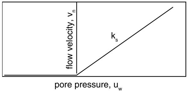# Defining drainage-only flow Drainage-only flow types can be specified for element-based or surface-based pore fluid flow to indicate that normal pore fluid flow occurs only from the interior to the exterior region of the model. The drainageonly flow surface condition assumes that the pore fluid flows in proportion to the magnitude of the current pore pressure on the surface, $u _ { w }$ , when that pressure is positive: $$ v _ {n} = k _ {s} u _ {w}, u _ {w} > 0 $$ $$ v _ {n} = 0, \quad u _ {w} \leq 0, $$ where Un $v _ { n }$ is the component of the pore fluid velocity in the direction of the outward normal to the surface; $k _ { s }$ is the seepage coefficient; and uw $u _ { w }$ is the current pore pressure at this point on the surface. Figure 34.4.7–1 illustrates this pore pressure–velocity relationship. This surface condition is designed for use with the total pore pressure formulation (see “Coupled pore fluid diffusion and stress analysis,” Section 6.8.1), mainly for cases where the phreatic surface intersects an exterior surface that is free to drain. See “Calculation of phreatic surface in an earth dam,” Section 10.1.2 of the Abaqus Example Problems Guide, for an example of this type of calculation. 

text_image

flow velocity, v_n k_s pore pressure, u_w

Figure 34.4.7–1 Drainage-only pore pressure–velocity relationship. When surface pore pressures are negative, the constraint will properly enforce the condition that no fluid can enter the interior region. When surface pore pressures are positive, the constraint will permit fluid flow from the interior to the exterior region of the model. When the seepage coefficient value, $k _ { s } ,$ , is large, this flow will approximately enforce the requirement that the pore pressure should be zero on a freely draining surface. To achieve this condition, it is necessary to choose the value of $k _ { s }$ to be much larger than a characteristic seepage coefficient for the material in the underlying elements: $$ k _ {s} \gg k / \gamma_ {w} c, $$ where $\pmb { k }$ is the permeability of the underlying material; $\gamma _ { w }$ is the fluid specific weight; and c is a characteristic length of the underlying elements. Values of $k _ { s } \approx 1 0 ^ { 5 } k / \gamma _ { w } c$ will be adequate for most analyses. Larger values of $k _ { s }$ could result in poor conditioning of the model. In all cases the freely draining flow type represents discontinuously nonlinear behavior, and its use may require appropriate solution controls (see “Commonly used control parameters,” Section 7.2.2). Input File Usage: Use the following option to define element-based drainage-only flow: \*FLOW element number or element set name, QnD, $k _ { s }$ Use the following option to define surface-based drainage-only flow: \*SFLOW surface name, QD, $k _ { s }$ Abaqus/CAE Usage: Pore fluid flow cannot be defined as a function of the current pore pressure in Abaqus/CAE. # Modifying or removing seepage coefficients and reference pore pressures Seepage coefficients and reference pore pressures can be added, modified, or removed as described in “Applying loads: overview,” Section 34.4.1. # Specifying a time-dependent reference pore pressure The magnitude of the reference pore pressure, $u _ { w } ^ { \infty }$ , can be controlled by referring to an amplitude curve. If different variations are needed for different portions of the flow, repeat the flow definition with each referring to its own amplitude curve. See “Applying loads: overview,” Section 34.4.1, and “Amplitude curves,” Section 34.1.2, for details. # Defining nonuniform flow in a user subroutine To define nonuniform flow, the variation of the reference pore pressure and the seepage coefficient as functions of position, time, pore pressure, etc. can be defined in user subroutine FLOW. ```txt Input File Usage: Use the following option to define a nonuniform element-based flow: *FLOW element number or element set name, QnNU Use the following option to define a nonuniform surface-based flow: *SFLOW surface name, QNU ``` Abaqus/CAE Usage: User subroutine FLOW is not supported in Abaqus/CAE. # Prescribing seepage flow velocity and seepage flow directly in consolidation analysis You can directly prescribe an outward normal flow velocity, $v _ { n }$ , across a surface or an outward normal flow at a node in consolidation analysis. # Prescribing element-based seepage flow velocity To prescribe an element-based seepage flow velocity, specify the element or element set name, the seepage type, and the outward normal flow velocity. The face of the element for which the seepage flow is being defined is identified by the seepage type. The seepage types available depend on the element type (see Part VI, “Elements”). Input File Usage: *DFLOW element number or element set name, Sn, $v_{n}$ Abaqus/CAE Usage: Load module: Create Load: choose Fluid for the Category and Surface pore fluid for the Types for Selected Step: select region: Distribution: select an analytical field, Magnitude: $v_{n}$