$$ \Delta \varepsilon_ {\alpha \beta} = \Delta \overline {{\varepsilon}} _ {\alpha \beta} + \overline {{f}} _ {3 3} ^ {t + \Delta t} S _ {3} \Delta \kappa_ {\alpha \beta}. $$ # Virtual work The virtual work contribution of the stresses is $$ \delta \Pi = \int_ {V} \sigma_ {\alpha \beta} \delta \varepsilon_ {\alpha \beta} d V. $$ We assume that the variations in the strain can be expressed in terms of variation in membrane strain and curvature with the same relations as apply to the increment in strain: $$ \delta \varepsilon_ {\alpha \beta} = \delta \overline {{\varepsilon}} _ {\alpha \beta} + \overline {{f}} _ {3 3} ^ {t + \Delta t} S _ {3} \delta \kappa_ {\alpha \beta}, $$ which transforms the virtual work equation into $$ \delta \Pi = \int_ {V} \sigma_ {\alpha \beta} (\delta \overline {{\varepsilon}} _ {\alpha \beta} + \overline {{f}} _ {3 3} S _ {3} \delta \kappa_ {\alpha \beta}) d V. $$ We introduce the membrane forces $N _ { \alpha \beta }$ and the bending moments $M _ { \alpha \beta }$ $$ N _ {\alpha \beta} \stackrel {\mathrm{def}} {=} \int_ {h} \sigma_ {\alpha \beta} \overline {{f}} _ {3 3} d S _ {3}, \qquad M _ {\alpha \beta} \stackrel {\mathrm{def}} {=} \int_ {h} \sigma_ {\alpha \beta} \overline {{f}} _ {3 3} ^ {2} S _ {3} \mathrm{d} S _ {3}, $$ which allows us to write $$ \delta \Pi = \int_ {A} \left(N _ {\alpha \beta} \delta \overline {{\varepsilon}} _ {\alpha \beta} + M _ {\alpha \beta} \delta \kappa_ {\alpha \beta}\right) d A. $$ The membrane strain variation follows with the usual expression $$ \delta \overline {{\varepsilon}} _ {\alpha \beta} = \mathrm{sym} (\delta \overline {{f}} _ {\alpha \gamma} \overline {{h}} _ {\gamma \beta}) = \mathrm{sym} (\delta \mathbf {t} _ {\alpha} \cdot \mathbf {t} _ {\beta} + \mathbf {t} _ {\alpha} \cdot \frac {\partial \delta \overline {{\mathbf {x}}}}{\partial s _ {\beta}}) = \mathrm{sym} (\mathbf {t} _ {\alpha} \cdot \frac {\partial \delta \overline {{\mathbf {x}}}}{\partial s _ {\beta}}), $$ where we have used the identity sym $\left( \delta \mathbf { t } _ { \alpha } \cdot \mathbf { t } _ { \beta } \right) = \delta ( \mathbf { t } _ { \alpha } \cdot \mathbf { t } _ { \beta } ) = 0$ . The variation in the curvature is obtained by taking variations in the incremental curvature, which yields $$ \begin{array}{l} \delta \kappa_ {\alpha \beta} = \mathrm{sym} (\epsilon_ {\alpha} ^ {\gamma} \mathbf {t} _ {\gamma} \cdot \delta \Delta \mathbf {r} _ {\beta} + \epsilon_ {\alpha} ^ {\gamma} \delta \mathbf {t} _ {\gamma} \cdot \Delta \mathbf {r} _ {\beta}) \\ = \mathrm{sym} (\epsilon_ {\alpha} ^ {\gamma} \mathbf {t} _ {\gamma} \cdot \delta \Delta \mathbf {R} _ {\delta} \overline {{h}} _ {\delta \beta} + \epsilon_ {\alpha} ^ {\gamma} \mathbf {t} _ {\gamma} \cdot \Delta \mathbf {R} _ {\delta} \delta \overline {{h}} _ {\delta \beta} + \epsilon_ {\alpha} ^ {\gamma} \delta \mathbf {t} _ {\gamma} \cdot \Delta \mathbf {R} _ {\delta} \overline {{h}} _ {\delta \beta}). \\ \end{array} $$ We neglect the terms of order $\Delta \kappa _ { \alpha \beta }$ and also terms of order $\mathbf { t } _ { 3 } \cdot \Delta \mathbf { r } _ { \delta }$ , which yields $$ \delta \kappa_ {\alpha \beta} = \mathrm{sym} (\epsilon_ {\alpha} ^ {\gamma} \mathbf {t} _ {\gamma} \cdot \delta \Delta \mathbf {r} _ {\delta} \overline {{h}} _ {\delta \beta}). $$ # Elements We evaluate $\delta \Delta \mathbf { r } _ { \delta }$ with respect to the current state (at the end of the increment). Hence for the evaluation we can assume $\Delta \phi = 0$ . Moreover, we neglect terms of the order $\mathbf { t } _ { \alpha } \cdot \frac { \partial \delta \Delta \phi } { \partial S _ { \beta } }$ @±¢Á @S¯ since they are proportional to $\Delta \kappa _ { \alpha \beta }$ . Hence, we obtain $$ \mathbf {t} _ {\gamma} \delta \Delta \mathbf {r} _ {\delta} \approx \mathbf {t} _ {\gamma} \cdot \frac {\partial \delta \pmb {\phi}}{\partial S _ {\delta}}, $$ which substituted in the expression for $\delta \kappa _ { \alpha \beta }$ yields $$ \delta \kappa_ {\alpha \beta} = \mathrm{sym} \left(\epsilon_ {\alpha} ^ {\gamma} \mathbf {t} _ {\gamma} \cdot \frac {\partial \delta \pmb {\phi}}{\partial S _ {\delta}} \overline {{h}} _ {\delta \beta}\right) = \mathrm{sym} \left(\epsilon_ {\alpha} ^ {\gamma} \mathbf {t} _ {\gamma} \cdot \frac {\partial \delta \pmb {\phi}}{\partial s _ {\beta}}\right). $$ # The rate of virtual work To obtain an expression for the rate of virtual work, we first write the virtual work equation in terms of the reference volume $$ \delta \Pi = \int_ {V ^ {\circ}} \tau_ {\alpha \beta} \delta \varepsilon_ {\alpha \beta} d V ^ {\circ} = \int_ {A ^ {\circ}} \int_ {h} \tau_ {\alpha \beta} \delta \varepsilon_ {\alpha \beta} d S _ {3} d A ^ {\circ}, $$ where $\tau _ { \alpha \beta }$ is the Kirchhoff stress tensor, related to the Cauchy or true stress tensor via $$ \tau_ {\alpha \beta} = J \sigma_ {\alpha \beta}. $$ The rate of change then becomes $$ \mathrm{d} \delta \Pi = \int_ {A ^ {\circ}} \int_ {h} (\mathrm{d} ^ {\nabla} \tau_ {\alpha \beta} \delta \varepsilon_ {\alpha \beta} + \tau_ {\alpha \beta} \mathrm{d} ^ {\nabla} \delta \varepsilon_ {\alpha \beta}) d S _ {3} d A ^ {\circ}. $$ Here $\mathrm { d } ^ { \nabla }$ indicates that the rates are taken in a material, corotational coordinate system. The terms involving stress rates are related to the material behavior. We assume constitutive equations of the form $$ \mathrm{d} ^ {\nabla} \tau_ {\alpha \beta} = J C _ {\alpha \beta \gamma \delta} \mathrm{d} \varepsilon_ {\delta \gamma}. $$ Substituted in the expression d±¦ and transformed back to the current configuration, this yields $$ \mathrm{d} \delta \Pi = \int_ {A} \int_ {h} \bigl (\delta \varepsilon_ {\alpha \beta} C _ {\alpha \beta \gamma \delta} \mathrm{d} \varepsilon_ {\gamma \delta} + \sigma_ {\alpha \beta} \mathrm{d} ^ {\nabla} \delta \varepsilon_ {\alpha \beta} \bigr) \overline {{f}} _ {3 3} d S _ {3} d A. $$ Consistent with the derivation of the virtual work equation itself, we neglect terms of the order $\mathrm { d } \overline { { f } } _ { 3 3 } S _ { 3 } \delta \kappa _ { \alpha \beta }$ . Hence, the rate of virtual work can be written as $$ \begin{array}{l} \mathrm{d} \delta \Pi = \int_ {A} \Big [ \int_ {h} (\delta \overline {{\varepsilon}} _ {\alpha \beta} + \overline {{f}} _ {3 3} S _ {3} \delta \kappa_ {\alpha \beta}) C _ {\alpha \beta \gamma \delta} (\mathrm{d} \overline {{\varepsilon}} _ {\gamma \delta} + \overline {{f}} _ {3 3} S _ {3} \mathrm{d} \kappa_ {\gamma \delta}) \overline {{f}} _ {3 3} d S _ {3} + \\ \left. N _ {\alpha \beta} \mathbf {d} ^ {\nabla} \delta \overline {{{\varepsilon}}} _ {\alpha \beta} + M _ {\alpha \beta} \mathbf {d} ^ {\nabla} \delta \kappa_ {\alpha \beta} \right] d A. \\ \end{array} $$ # Second variation of the membrane strain It remains to determine $\mathrm { d } ^ { \nabla } \delta \overline { { \varepsilon } } _ { \alpha \beta }$ and $\mathrm { d } ^ { \nabla } \delta \kappa _ { \alpha \beta }$ . From the first variation $\delta \overline { { \mathcal { E } } } _ { \alpha \beta }$ follows $$ \mathrm{d} ^ {\nabla} \delta \overline {{\varepsilon}} _ {\alpha \beta} = \mathrm{sym} (\mathrm{d} ^ {\nabla} \delta \overline {{f}} _ {\alpha \gamma} \overline {{h}} _ {\gamma \beta} + \delta \overline {{f}} _ {\alpha \gamma} \mathrm{d} ^ {\nabla} \overline {{h}} _ {\gamma \beta}). $$ Since $\overline { { h } } _ { \alpha \beta }$ is the inverse of $\overline { { f } } _ { \alpha \beta }$ , it follows that $$ \mathrm{d} ^ {\nabla} \overline {{h}} _ {\alpha \beta} = - \overline {{h}} _ {\alpha \gamma} \mathrm{d} ^ {\nabla} \overline {{f}} _ {\gamma \delta} \overline {{h}} _ {\delta \beta}. $$ Substitution in the expression for the second variation yields $$ \begin{array}{l} \mathrm{d} ^ {\nabla} \delta \overline {{\varepsilon}} _ {\alpha \beta} = \mathrm{sym} \left(\mathrm{d} ^ {\nabla} \mathbf {t} _ {\alpha} \cdot \frac {\partial \delta \overline {{\mathbf {x}}}}{\partial s _ {\beta}} - \mathbf {t} _ {\alpha} \cdot \frac {\partial \delta \overline {{\mathbf {x}}}}{\partial s _ {\gamma}} \mathrm{d} ^ {\nabla} \mathbf {t} _ {\gamma} \cdot \frac {\partial \overline {{\mathbf {x}}}}{\partial s _ {\beta}} - \mathbf {t} _ {\alpha} \cdot \frac {\partial \delta \overline {{\mathbf {x}}}}{\partial s _ {\gamma}} \mathbf {t} _ {\gamma} \cdot \frac {\partial \mathrm{d} ^ {\nabla} \overline {{\mathbf {x}}}}{\partial s _ {\beta}}\right) \\ = \mathrm{sym} \left(\mathrm{d} ^ {\nabla} \mathbf {t} _ {\alpha} \cdot \frac {\partial \delta \overline {{\mathbf {x}}}}{\partial s _ {\beta}} - \mathrm{d} ^ {\nabla} \mathbf {t} _ {\gamma} \cdot \mathbf {t} _ {\beta} \mathbf {t} _ {\alpha} \cdot \frac {\partial \delta \overline {{\mathbf {x}}}}{\partial s _ {\gamma}} - \frac {\partial \mathrm{d} ^ {\nabla} \overline {{\mathbf {x}}}}{\partial s _ {\beta}} \cdot \mathbf {t} _ {\gamma} \mathbf {t} _ {\alpha} \cdot \frac {\partial \delta \overline {{\mathbf {x}}}}{\partial s _ {\gamma}}\right). \\ \end{array} $$ The corotational rate of the base vectors follows from $$ \mathbf {d} ^ {\nabla} \mathbf {t} _ {\beta} = \frac {\partial \mathrm{d} \overline {{\mathbf {x}}}}{\partial s _ {\beta}} + \frac {\partial \overline {{\mathbf {x}}}}{\partial S _ {\gamma}} \mathbf {d} ^ {\nabla} \overline {{h}} _ {\gamma \beta} = \frac {\partial \mathrm{d} \overline {{\mathbf {x}}}}{\partial s _ {\beta}} - \mathbf {d} ^ {\nabla} \mathbf {t} _ {\gamma} \cdot \mathbf {t} _ {\beta} \mathbf {t} _ {\gamma} - \frac {\partial \mathrm{d} \overline {{\mathbf {x}}}}{\partial s _ {\beta}} \cdot \mathbf {t} _ {\gamma} \mathbf {t} _ {\gamma}. $$ Substituted in the first term of the previous expression yields $$ \begin{array}{l} \mathrm{d} ^ {\nabla} \delta \overline {{{\varepsilon}}} _ {\alpha \beta} = \mathrm{sym} \bigg [ \frac {\partial \mathrm{d} \overline {{{\mathbf {x}}}}}{\partial s _ {\alpha}} \cdot \frac {\partial \delta \overline {{{\mathbf {x}}}}}{\partial s _ {\beta}} - \mathrm{d} ^ {\nabla} \mathbf {t} _ {\gamma} \cdot \mathbf {t} _ {\alpha} \mathbf {t} _ {\gamma} \cdot \frac {\partial \delta \overline {{{\mathbf {x}}}}}{\partial s _ {\beta}} - \mathrm{d} ^ {\nabla} \mathbf {t} _ {\gamma} \cdot \mathbf {t} _ {\beta} \mathbf {t} _ {\alpha} \cdot \frac {\partial \delta \overline {{{\mathbf {x}}}}}{\partial s _ {\gamma}} - \mathrm{d} ^ {\nabla} \mathbf {t} _ {\gamma} \cdot \mathbf {t} _ {\beta} \mathbf {t} _ {\alpha} \cdot \frac {\partial \delta \overline {{{\mathbf {x}}}}}{\partial s _ {\beta}} \bigg ] \\ \left. \frac {\partial \mathrm{d} \overline {{{\mathbf {x}}}}}{\partial s _ {\alpha}} \cdot \mathbf {t} _ {\gamma} \mathbf {t} _ {\gamma} \cdot \frac {\partial \delta \overline {{{\mathbf {x}}}}}{\partial s _ {\beta}} - \frac {\partial \mathrm{d} \overline {{{\mathbf {x}}}}}{\partial s _ {\beta}} \cdot \mathbf {t} _ {\gamma} \mathbf {t} _ {\alpha} \cdot \frac {\partial \delta \overline {{{\mathbf {x}}}}}{\partial s _ {\gamma}} \right] \\ = \mathrm{sym} \left[ \frac {\partial \mathrm{d} \overline {{{\mathbf {x}}}}}{\partial s _ {\alpha}} \cdot \frac {\partial \delta \overline {{{\mathbf {x}}}}}{\partial s _ {\beta}} - 2 \left(\mathrm{d} ^ {\nabla} \mathbf {t} _ {\gamma} \cdot \mathbf {t} _ {\alpha} + \frac {\partial \mathrm{d} \overline {{{\mathbf {x}}}}}{\partial s _ {\alpha}} \cdot \mathbf {t} _ {\gamma}\right) \delta \overline {{{\varepsilon}}} _ {\gamma \beta} \right]. \\ \end{array} $$ The in-plane components of the corotational rate of the base vectors can also be expressed in terms of the in-plane material spin in the reference surface: $$ \mathrm{d} ^ {\nabla} \mathbf {t} _ {\gamma} = \mathrm{d} \Omega_ {\gamma \beta} \mathbf {t} _ {\beta} = \frac {1}{2} \left(\mathbf {t} _ {\beta} \cdot \frac {\partial \mathrm{d} \overline {{\mathbf {x}}}}{\partial s _ {\gamma}} - \mathbf {t} _ {\gamma} \cdot \frac {\partial \mathrm{d} \overline {{\mathbf {x}}}}{\partial s _ {\beta}}\right) \mathbf {t} _ {\beta}. $$ Substitution in the last obtained expression for $\mathrm { d } ^ { \nabla } \delta \overline { { \varepsilon } } _ { \alpha \beta }$ yields $$ \mathrm{d} ^ {\nabla} \delta \overline {{\varepsilon}} _ {\alpha \beta} = \mathrm{sym} \left(\frac {\partial \mathrm{d} \overline {{\mathbf {x}}}}{\partial s _ {\alpha}} \cdot \frac {\partial \delta \overline {{\mathbf {x}}}}{\partial s _ {\beta}} - 2 \mathrm{d} \overline {{\varepsilon}} _ {\alpha \gamma} \delta \overline {{\varepsilon}} _ {\gamma \beta}\right). $$ This expression is identical to the one obtained with "standard" continuum elements. # Second variation of the curvature We need to calculate the second variation of the curvature to calculate the initial stress contribution from the curvature: $$ m ^ {\alpha \beta} \mathrm{d} ^ {\nabla} \delta \kappa_ {\alpha \beta}. $$ To simplify the computation, we rely on the intrinsic definition of curvature and express the curvature in derivatives with respect to the isoparametric coordinates. Accordingly, $$ m ^ {\alpha \beta} \mathrm{d} ^ {\nabla} \delta \kappa_ {\alpha \beta} = m ^ {a b} \mathrm{d} ^ {\nabla} \delta \kappa_ {a b} = m ^ {a b} \mathrm{d} ^ {\nabla} \left(\frac {\partial \delta \overline {{\mathbf {x}}}}{\partial \xi^ {a}} \cdot \frac {\partial \mathbf {t} _ {3}}{\partial \xi^ {b}} + \frac {\partial \overline {{\mathbf {x}}}}{\partial \xi^ {a}} \cdot \frac {\partial \delta \mathbf {t} _ {3}}{\partial \xi^ {b}}\right), $$ where the bending resultant components $m ^ { a b }$ are the components expressed in the orthonormal coordinate system $( m ^ { \alpha \beta } )$ transformed by $\partial \xi ^ { a } / \partial s _ { \alpha }$ . Denoting derivatives with respect to the isoparametric coordinates as $\partial / \partial \xi ^ { a } \equiv { , } a$ , the second variation of the curvature is $$ \mathrm{d} ^ {\nabla} \delta \kappa_ {a b} = \delta \overline {{\mathbf {x}}} _ {, a} \cdot \mathrm{d} ^ {\nabla} \mathbf {t} _ {3, b} + \mathrm{d} \overline {{\mathbf {x}}} _ {, a} \cdot \delta \mathbf {t} _ {3, b} + \overline {{\mathbf {x}}} _ {, a} \cdot (\mathrm{d} ^ {\nabla} \delta \mathbf {t} _ {3}) _ {, b}. $$ Using the fact that $\delta \mathbf { t } _ { 3 } = \delta { \pmb { \phi } } \times \mathbf { t } _ { 3 }$ and $\mathbf { d } ^ { \nabla } \mathbf { t } _ { 3 } = \pmb { \phi } \times \mathbf { t } _ { 3 }$ , we find that $$ \begin{array}{l} \mathrm{d} ^ {\nabla} \delta \kappa_ {a b} = \delta \overline {{\mathbf {x}}} _ {, a} \cdot [ - \hat {\mathbf {t}} _ {3} ] \cdot \dot {\pmb {\phi}} _ {, b} + \delta \overline {{\mathbf {x}}} _ {, a} \cdot [ - \hat {\mathbf {t}} _ {3, b} ] \cdot \dot {\pmb {\phi}} + \delta \pmb {\phi} _ {, b} \cdot [ \hat {\mathbf {t}} _ {3} ] \cdot \mathrm{d} \overline {{\mathbf {x}}} _ {, a} + \delta \pmb {\phi} \cdot [ \hat {\mathbf {t}} _ {3, b} ] \cdot \mathrm{d} \overline {{\mathbf {x}}} _ {, a} \\ + \delta \pmb {\phi} _ {, b} \cdot (\mathbf {t} _ {3} \overline {{\mathbf {x}}} _ {, a}) \cdot \pmb {\phi} + \delta \pmb {\phi} \cdot (\mathbf {t} _ {3, b} \overline {{\mathbf {x}}} _ {, a}) \cdot \pmb {\phi} + \delta \pmb {\phi} \cdot (\mathbf {t} _ {3} \overline {{\mathbf {x}}} _ {, a}) \cdot \pmb {\phi} _ {, b} \\ - \delta \boldsymbol {\phi} _ {, b} \cdot (\mathbf {t} _ {3} \cdot \overline {{\mathbf {x}}} _ {, a} \mathbf {I}) \cdot \boldsymbol {\phi} - \delta \boldsymbol {\phi} \cdot (\mathbf {t} _ {3} \cdot \overline {{\mathbf {x}}} _ {, a} \mathbf {I}) \cdot \boldsymbol {\phi} _ {, b} - \delta \boldsymbol {\phi} \cdot (\mathbf {t} _ {3, b} \cdot \overline {{\mathbf {x}}} _ {, a} \mathbf {I}) \cdot \boldsymbol {\phi}. \\ \end{array} $$ Here $[ \hat { \bf t } _ { 3 } ]$ indicates the skew-symmetric tensor with axial vector $\mathbf { t } _ { 3 }$ # Transverse shear treatment Several interpolation schemes have been proposed to avoid shear-locking, which typically arises as the thickness of a plate or shell goes to zero. Here we employ an assumed strain method based on the Hu-Washizu principle. This scheme derives from that by MacNeal (1978), subsequently extended and reformulated in Hughes and Tezduyar (1981) and MacNeal (1982) and revisited in Bathe and Dvorkin (1984). Computational aspects of the nonlinear theory are investigated in Simo, Fox, and Rifai (1989) for fully integrated quadrilateral shell elements. For reduced integration quadrilateral and triangular shell elements that can be used for both implicit and explicit integration, this assumed strain method needs to be modified. We summarize below the assumed strain method used with fully integrated elements, followed by the modifications required for the one-point integration plus stabilization used in ABAQUS. 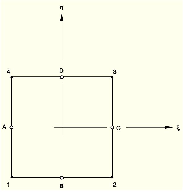# Construction of the assumed strain field Consider a typical isoparametric finite element, as depicted in Figure 3.6.5-1, and denote by A; B; C; D the set of midpoints of the element boundaries. Figure 3.6.5-1 Notation for the assumed strain field on the standard isoparametric element. 

text_image

η 4 D 3 A C ξ 1 B 2

The following assumed transverse shear strain field is used: $$ \overline {{\gamma}} _ {1} = \frac {1}{2} \left[ (1 - \eta) \gamma_ {1} ^ {B} + (1 + \eta) \gamma_ {1} ^ {D} \right] $$ $$ \overline {{\gamma}} _ {2} = \frac {1}{2} \left[ (1 - \xi) \gamma_ {2} ^ {A} + (1 + \xi) \gamma_ {2} ^ {C} \right], $$ where $$ \gamma_ {2} ^ {A} = \mathbf {t} ^ {A} \cdot \overline {{\mathbf {x}}} _ {, 2} ^ {A} - \mathbf {T} ^ {A} \cdot \overline {{\mathbf {X}}} _ {, 2} ^ {A}, \quad \gamma_ {1} ^ {B} = \mathbf {t} ^ {B} \cdot \overline {{\mathbf {x}}} _ {, 1} ^ {B} - \mathbf {T} ^ {B} \cdot \overline {{\mathbf {X}}} _ {, 1} ^ {B}, $$ $$ \gamma_ {2} ^ {C} = \mathbf {t} ^ {C} \cdot \overline {{\mathbf {x}}} _ {, 2} ^ {C} - \mathbf {T} ^ {C} \cdot \overline {{\mathbf {X}}} _ {, 2} ^ {C}, \quad \gamma_ {1} ^ {D} = \mathbf {t} ^ {D} \cdot \overline {{\mathbf {x}}} _ {, 1} ^ {D} - \mathbf {T} ^ {D} \cdot \overline {{\mathbf {X}}} _ {, 1} ^ {D} $$ are the covariant transverse shear strains evaluated at the midpoints of the element boundaries. In the above transverse shear strain definitions, the use of uppercase letters indicates quantities in the reference configuration and the use of lowercase letters indicates the deformed configuration. For readability we have omitted the subscript 3 from the director field. Making use of the bilinear element interpolation, it follows that # Elements $$ \overline {{\mathbf {x}}} _ {, 2} ^ {A} = \frac {1}{2} \big (\overline {{\mathbf {x}}} _ {4} - \overline {{\mathbf {x}}} _ {1} \big), \quad \overline {{\mathbf {x}}} _ {, 1} ^ {B} = \frac {1}{2} \big (\overline {{\mathbf {x}}} _ {2} - \overline {{\mathbf {x}}} _ {1} \big), $$ $$ \overline {{{\mathbf {x}}}} _ {, 2} ^ {C} = \frac {1}{2} \big (\overline {{{\mathbf {x}}}} _ {3} - \overline {{{\mathbf {x}}}} _ {2} \big), \qquad \qquad \overline {{{\mathbf {x}}}} _ {, 1} ^ {D} = \frac {1}{2} \big (\overline {{{\mathbf {x}}}} _ {3} - \overline {{{\mathbf {x}}}} _ {4} \big), $$ where $\overline { { \mathbf { x } } } _ { I }$ , for $I = 1 , 2 , 3 , 4$ , are the reference surface position vectors of the element nodes. By making use of the assumed strain field along with the update formulae for the director field, the assumed covariant transverse shear field can be written concisely in matrix notation. Recall the director field update equation and the corresponding linearized director field: $$ \mathbf {t} _ {t + \Delta t} = \exp [ \hat {\Delta \phi} ] \cdot \mathbf {t} _ {t} \quad \Rightarrow \quad \delta \mathbf {t} = \delta \boldsymbol {\phi} \times \mathbf {t}. $$ It follows from the element interpolation that $$ \delta \mathbf {t} ^ {A} = \frac {1}{2} (\delta \pmb {\phi} _ {4} + \delta \pmb {\phi} _ {1}) \times \mathbf {t} ^ {A}, \qquad \delta \mathbf {t} ^ {B} = \frac {1}{2} (\delta \pmb {\phi} _ {2} + \delta \pmb {\phi} _ {1}) \times \mathbf {t} ^ {B}, $$ $$ \delta \mathbf {t} ^ {C} = \frac {1}{2} (\delta \pmb {\phi} _ {3} + \delta \pmb {\phi} _ {2}) \times \mathbf {t} ^ {C}, \delta \mathbf {t} ^ {D} = \frac {1}{2} (\delta \pmb {\phi} _ {3} + \delta \pmb {\phi} _ {4}) \times \mathbf {t} ^ {D}. $$ Define the following vectors: $$ \overline {{\boldsymbol {\gamma}}} = \left\{\overline {{\gamma}} _ {1} \atop \overline {{\gamma}} _ {2} \right\}, \delta \overline {{\mathbf {x}}} = \left\{ \begin{array}{l} \delta \overline {{\mathbf {x}}} _ {1} \\ \delta \overline {{\mathbf {x}}} _ {2} \\ \delta \overline {{\mathbf {x}}} _ {3} \\ \delta \overline {{\mathbf {x}}} _ {4} \end{array} \right\}, \delta \boldsymbol {\phi} = \left\{ \begin{array}{l} \delta \boldsymbol {\phi} _ {1} \\ \delta \boldsymbol {\phi} _ {2} \\ \delta \boldsymbol {\phi} _ {3} \\ \delta \boldsymbol {\phi} _ {4} \end{array} \right\}. $$ Then, the linearized transverse shear strain is $$ \delta \overline {{\boldsymbol {\gamma}}} \equiv \left\{ \begin{array}{l} \delta \overline {{\boldsymbol {\gamma}}} _ {1} \\ \delta \overline {{\boldsymbol {\gamma}}} _ {2} \end{array} \right\} = \bar {B} _ {s m} \delta \overline {{\mathbf {x}}} + \bar {B} _ {s b} \delta \boldsymbol {\phi}, $$ where $$ \bar {B} _ {s m} = \frac {1}{4} \left[ \begin{array}{c c c c} - (1 - \eta) \mathbf {t} ^ {B ^ {T}} & (1 - \eta) \mathbf {t} ^ {B ^ {T}} & (1 + \eta) \mathbf {t} ^ {D ^ {T}} & - (1 + \eta) \mathbf {t} ^ {D ^ {T}} \\ - (1 - \xi) \mathbf {t} ^ {A ^ {T}} & - (1 + \xi) \mathbf {t} ^ {C ^ {T}} & (1 + \xi) \mathbf {t} ^ {C ^ {T}} & (1 - \xi) \mathbf {t} ^ {A ^ {T}} \end{array} \right]. $$ Define the four vectors: $$ \pmb {\eta} _ {2} ^ {A} = \mathbf {t} ^ {A} \times \overline {{\mathbf {x}}} _ {, 2} ^ {A}, \qquad \pmb {\eta} _ {1} ^ {B} = \mathbf {t} ^ {B} \times \overline {{\mathbf {x}}} _ {, 1} ^ {B}, $$ $$ \boldsymbol {\eta} _ {2} ^ {C} = \mathbf {t} ^ {C} \times \overline {{\mathbf {x}}} _ {, 2} ^ {C}, \quad \boldsymbol {\eta} _ {1} ^ {D} = \mathbf {t} ^ {D} \times \overline {{\mathbf {x}}} _ {, 1} ^ {D}. $$ Then the rotation or bending part of the strain/displacement operator is written $$ \bar {B} _ {s b} = \frac {1}{4} \left[ \begin{array}{c c c c} (1 - \eta) \pmb {\eta} _ {1} ^ {B ^ {T}} & (1 - \eta) \pmb {\eta} _ {1} ^ {B ^ {T}} & (1 + \eta) \pmb {\eta} _ {1} ^ {D ^ {T}} & (1 + \eta) \pmb {\eta} _ {1} ^ {D ^ {T}} \\ (1 - \xi) \pmb {\eta} _ {2} ^ {A ^ {T}} & (1 + \xi) \pmb {\eta} _ {2} ^ {C ^ {T}} & (1 + \xi) \pmb {\eta} _ {2} ^ {C ^ {T}} & (1 - \xi) \pmb {\eta} _ {2} ^ {A ^ {T}} \end{array} \right]. $$ # Elements # Constitutive relations A St. Venant-Kirchhoff constitutive model for the Kirchhoff curvilinear components of the resultant transverse shear force is written in terms of the transverse shear strains as $$ \left\{ \begin{array}{l} Q ^ {1} \\ Q ^ {2} \end{array} \right\} = \mathbf {C} _ {s} \left\{ \begin{array}{l} \overline {{\gamma}} _ {1} \\ \overline {{\gamma}} _ {2} \end{array} \right\}, $$ where $\mathbf { C } _ { s }$ is the transverse shear stiffness in curvilinear coordinates. For a single isotropic layer, $$ \mathbf {C} _ {s} = \frac {5}{6} G _ {s} h \left[ \begin{array}{c c} A ^ {1 1} & A ^ {1 2} \\ A ^ {2 1} & A ^ {2 2} \end{array} \right]. $$ The matrix $\big [ A ^ { \alpha \beta } \big ]$ is the inverse of the metric $[ A _ { \alpha \beta } ]$ , where metric components in the reference configuration $A _ { \alpha \beta }$ are defined by the inner product $$ A _ {\alpha \beta} = \overline {{\mathbf {X}}} _ {, \alpha} \cdot \overline {{\mathbf {X}}} _ {, \beta}. $$ The Cauchy or true transverse shear force components in the shell orthonormal coordinate system $\{ q ^ { 1 } , q ^ { 2 } \} ^ { T }$ are calculated with the coordinate transformation $f _ { \alpha } ^ { a } = \partial s ^ { a } / \partial \xi ^ { \alpha }$ as $$ \mathbf {q} = \left\{ \begin{array}{l} q ^ {1} \\ q ^ {2} \end{array} \right\} = \frac {A}{a} \left[ \begin{array}{l l} f _ {1} ^ {1} & f _ {2} ^ {1} \\ f _ {1} ^ {2} & f _ {2} ^ {2} \end{array} \right] \left\{ \begin{array}{l} Q ^ {1} \\ Q ^ {2} \end{array} \right\}, $$ where A is the element's reference area and a is the current area. # Initial stress stiffness The calculation of the initial stress stiffness matrix requires the second variation of the assumed transverse strain field. This calculation can be summarized in matrix notation as follows. Define vectors of variations of the nodal displacement quantities: $$ \delta \mathbf {u} = \left\{ \begin{array}{l} \delta \overline {{\mathbf {x}}} _ {1} \\ \delta \pmb {\phi} _ {1} \\ \delta \overline {{\mathbf {x}}} _ {2} \\ \delta \pmb {\phi} _ {2} \\ \delta \overline {{\mathbf {x}}} _ {3} \\ \delta \pmb {\phi} _ {3} \\ \delta \overline {{\mathbf {x}}} _ {4} \\ \delta \pmb {\phi} _ {4} \end{array} \right\}, \quad \mathrm{d} \mathbf {u} = \left\{ \begin{array}{l} \mathrm{d} \overline {{\mathbf {x}}} _ {1} \\ \mathrm{d} \pmb {\phi} _ {1} \\ \mathrm{d} \overline {{\mathbf {x}}} _ {2} \\ \mathrm{d} \pmb {\phi} _ {2} \\ \mathrm{d} \overline {{\mathbf {x}}} _ {3} \\ \mathrm{d} \pmb {\phi} _ {3} \\ \mathrm{d} \overline {{\mathbf {x}}} _ {4} \\ \mathrm{d} \pmb {\phi} _ {4} \end{array} \right\}. $$ Then the initial stress contribution is written $$ \mathbf {q} \cdot \mathrm{d} \delta \bar {\boldsymbol {\gamma}} = \int \delta \mathbf {u} \cdot \mathbf {K} _ {s} \cdot \Delta \mathbf {u} d a, $$ # Elements where da is the area measure in the current configuration and ${ \bf K } _ { s }$ is the (symmetric) transverse shear contribution to the initial stress, defined as follows. Let I be the $3 \times 3$ identity matrix; then define the symmetric matrices $$ \mathbf {A} = Q ^ {2} (1 - \xi) \left[ \mathrm{sym} \{\mathbf {t} ^ {A} (\overline {{\mathbf {x}}} _ {, 2} ^ {A}) ^ {T} \} - \gamma_ {2} ^ {A} \mathbf {I} \right], \quad \mathbf {B} = Q ^ {1} (1 - \eta) \left[ \mathrm{sym} \{\mathbf {t} ^ {B} (\overline {{\mathbf {x}}} _ {, 1} ^ {B}) ^ {T} \} - \gamma_ {1} ^ {B} \mathbf {I} \right], $$ $$ \mathbf {C} = Q ^ {2} (1 + \xi) \left[ \mathrm{sym} \{\mathbf {t} ^ {C} (\overline {{\mathbf {x}}} _ {, 2} ^ {C}) ^ {T} \} - \gamma_ {2} ^ {C} \mathbf {I} \right], \quad \mathbf {D} = Q ^ {1} (1 + \eta) \left[ \mathrm{sym} \{\mathbf {t} ^ {D} (\overline {{\mathbf {x}}} _ {, 1} ^ {D}) ^ {T} \} - \gamma_ {1} ^ {D} \mathbf {I} \right]. $$ Also define the skew-symmetric matrices $$ \hat {\mathbf {a}} = Q ^ {2} (1 - \xi) \hat {\mathbf {t}} ^ {A}, \quad \hat {\mathbf {b}} = Q ^ {1} (1 - \eta) \hat {\mathbf {t}} ^ {B}, $$ $$ \hat {\mathbf {c}} = Q ^ {2} (1 + \xi) \hat {\mathbf {t}} ^ {C}, \quad \hat {\mathbf {d}} = Q ^ {1} (1 + \eta) \hat {\mathbf {t}} ^ {D}. $$ Also, let 0 be the $3 \times 3$ zero matrix. Then ${ \bf K } _ { s }$ is written $$ \mathbf {K} _ {s} = \frac {1}{8} \left[ \begin{array}{c c c c c c c c} \mathbf {0} & \hat {\mathbf {a}} + \hat {\mathbf {b}} & \mathbf {0} & \hat {\mathbf {b}} & \mathbf {0} & \mathbf {0} & & \hat {\mathbf {a}} \\ - \hat {\mathbf {a}} - \hat {\mathbf {b}} & \mathbf {A} + \mathbf {B} & \hat {\mathbf {b}} & \mathbf {B} & \mathbf {0} & \mathbf {0} & \hat {\mathbf {a}} & \mathbf {A} \\ \mathbf {0} & - \hat {\mathbf {b}} & \mathbf {0} & - \hat {\mathbf {b}} + \hat {\mathbf {c}} & \mathbf {0} & \hat {\mathbf {c}} & \mathbf {0} & \mathbf {0} \\ - \hat {\mathbf {b}} & \mathbf {B} & \hat {\mathbf {b}} - \hat {\mathbf {c}} & \mathbf {B} + \mathbf {C} & \hat {\mathbf {c}} & \mathbf {C} & \mathbf {0} & \mathbf {0} \\ \mathbf {0} & \mathbf {0} & \mathbf {0} & - \hat {\mathbf {c}} & \mathbf {0} & - \hat {\mathbf {c}} - \hat {\mathbf {d}} & \mathbf {0} & - \hat {\mathbf {d}} \\ \mathbf {0} & \mathbf {0} & - \hat {\mathbf {c}} & \mathbf {C} & \hat {\mathbf {c}} + \hat {\mathbf {d}} & \mathbf {C} + \mathbf {D} & - \hat {\mathbf {d}} & \mathbf {D} \\ \mathbf {0} & - \hat {\mathbf {a}} & \mathbf {0} & \mathbf {0} & \mathbf {0} & \hat {\mathbf {d}} & \mathbf {0} & \hat {\mathbf {d}} - \hat {\mathbf {a}} \\ - \hat {\mathbf {a}} & \mathbf {A} & \mathbf {0} & \mathbf {0} & \hat {\mathbf {d}} & \mathbf {D} & - \hat {\mathbf {d}} + \hat {\mathbf {a}} & \mathbf {D} + \mathbf {A} \end{array} \right]. $$ # One point integration plus stabilization For reduced integration elements the transverse shear force components need to be evaluated at the center of the elements. Consider $\pi _ { s }$ the transverse shear contribution to the internal energy: $$ \pi_ {s} = \frac {1}{2} \int \overline {{{\boldsymbol {\gamma}}}} \cdot \mathbf {C} _ {s} \cdot \overline {{{\boldsymbol {\gamma}}}} d A. $$ The reference area measure dA is written in terms of the isoparametric coordinates as $d A = J d \xi d \eta$ , where $J = \sqrt { A _ { 1 1 } A _ { 2 2 } - ( A _ { 1 2 } ) ^ { 2 } }$ and $A _ { \alpha \beta }$ are the components of the reference surface metric in the undeformed configuration. This transverse shear energy can be approximated in many ways to produce a one point integration at the center of the element plus hourglass stabilization. It is important that this treatment yield accurate representation of transverse shear deformation in thick shell problems and provide robust performance for skewed elements. The treatment should collapse smoothly to a triangle, which should be insensitive to the node numbering during collapse; that is, the triangle's response should not depend on the nodal connectivity. For an entire mesh of triangular elements, the treatment should give convergent results (that is, the element should not lock). Furthermore, the high frequency response of the transverse shear treatment should be controlled so that transverse shear response does not dominate the stable time increment for explicit dynamic analysis (including for skewed triangular or quadrilateral geometries). # Elements All of these requirements are embodied in the following transverse shear treatment. Define the transverse shear strain at the center of the element (the homogeneous part) and the "hourglass" transverse shear strain vectors as $$ \overline {{\gamma}} _ {0} = \frac {1}{2} \left\{ \begin{array}{l} \gamma_ {1} ^ {B} + \gamma_ {1} ^ {D} \\ \gamma_ {2} ^ {A} + \gamma_ {2} ^ {C} \end{array} \right\} + \gamma_ {c c} \left\{ \begin{array}{l} c _ {\xi} \\ c _ {\eta} \end{array} \right\} \quad \mathrm{and} \quad \gamma_ {h g} = \left\{ \begin{array}{l} \gamma_ {b f} \\ \gamma_ {c c} \end{array} \right\}. $$ The element distortion coefficients $c _ { \xi }$ and $c _ { \eta }$ are constants determined by the element reference geometry. For geometries with constant Jacobian transformation, $c _ { \xi } = c _ { \eta } = 0$ . The components of the hourglass strain vector $\gamma _ { h g }$ are defined in terms of the edge strains as $$ \gamma_ {b f} = - \Gamma_ {A} \gamma_ {2} ^ {A} + \Gamma_ {B} \gamma_ {1} ^ {B} + \Gamma_ {C} \gamma_ {2} ^ {C} - \Gamma_ {D} \gamma_ {1} ^ {D} \quad \mathrm{and} \quad \gamma_ {c c} = - \gamma_ {2} ^ {A} + \gamma_ {1} ^ {B} + \gamma_ {2} ^ {C} - \gamma_ {1} ^ {D}. $$ The coefficients $\Gamma _ { A } , \Gamma _ { B } , \Gamma _ { C }$ , and $\Gamma _ { D }$ are constants determined from the reference geometry of the element. For rectangular elements $\Gamma _ { A } = { \textstyle { \frac { 1 } { 2 } } } , \Gamma _ { B } = - { \textstyle { \frac { 1 } { 2 } } } , \Gamma _ { C } = { \textstyle { \frac { 1 } { 2 } } } , \Gamma _ { D } = - { \textstyle { \frac { 1 } { 2 } } }$ ; and $\gamma _ { b f }$ can be identified as the strain associated with the rotational "butterfly" deformation pattern. We call $\gamma _ { c c }$ the "crop circle" mode strain since it corresponds to a deformation pattern that resembles the sweeping over the element normals in a circular pattern. The inclusion of the crop circle strain $\gamma _ { c c }$ in the homogeneous part of the transverse shear strain $\bar { \gamma } _ { 0 }$ has two important consequences. First, it makes the transverse shear response insensitive to the nodal connectivity for a triangular element. That is, when a side of a quadrilateral element is collapsed to form a triangle, the element's response is independent of the choice of node numbering on the element. Second, for explicit dynamic analyses the coefficients $c _ { \xi }$ and $c _ { \eta }$ are chosen to minimize the highest frequencies associated with the homogeneous part of the transverse shear response. 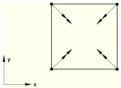To illustrate the crop circle and butterfly transverse shear patterns, consider a square, initially flat element. Furthermore, consider plate theory kinematics; that is, two rotations and a vertical deflection at the nodes. The crop circle pattern has zero vertical deflection at the nodes and a nodal rotation vector pattern as illustrated in Figure 3.6.5-2. Figure 3.6.5-2 Crop circle pattern: zero deflection and circularly symmetric rotations. 

text_image

y x

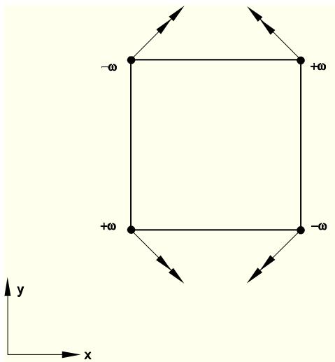
The butterfly pattern has vertical deflections that correspond to cross-diagonal bending; that is, two equal deflections at two nodes across a diagonal, with equal and opposite deflections at the remaining # Elements two nodes. The nodal rotations develop in a way that opposes the bending motion of the reference surface; that is, the rotations are opposite the rotations that would develop for this displacement pattern to produce pure bending. The butterfly mode's nodal vertical deflection and rotation vector pattern are illustrated in Figure 3.6.5-3. Figure 3.6.5-3 Butterfly pattern: vertical deflection and rotation vectors. 

text_image

-ω +ω +ω -ω y x

Let the reference element area be $A _ { 0 } = 4 J _ { 0 }$ . The transverse shear energy can be approximated as a center point value plus a stabilization term: $$ \pi_ {s} = \frac {1}{2} A _ {0} \overline {{\boldsymbol {\gamma}}} _ {0} \cdot \mathbf {C} _ {s 0} \cdot \overline {{\boldsymbol {\gamma}}} _ {0} + \frac {1}{2} A _ {0} \boldsymbol {\gamma} _ {h g} \cdot \mathbf {H} \cdot \boldsymbol {\gamma} _ {h g}, $$ where $\mathbf { C } _ { s 0 }$ is the transverse shear stiffness evaluated at the center of the element and the hourglass stiffness H is the diagonal matrix $$ \mathbf {H} = \frac {C _ {s 0} ^ {e f f}}{1 2} \left[ \begin{array}{c c} 1 & 0 \\ 0 & 0. 0 0 1 \end{array} \right]. $$ The effective stiffness $C _ { s 0 } ^ { e f f }$ is the average direct component of the transverse shear stiffness, $C _ { s 0 } ^ { e f f } = ( C _ { s 0 } ^ { 1 1 } + C _ { s 0 } ^ { 2 2 } ) / 2$ . The formulation of the homogeneous part of the transverse shear has two contributions: the average edge strain across the element, plus the element distortion term. The average strain treatment is essentially the same as that for the assumed strain formulation of MacNeal and others presented earlier, with expressions evaluated at the center of the element $( \xi = 0$ and $\eta = 0 )$ . The details of this part are omitted; only the element distortion term is presented in detail. The variation of the homogeneous transverse shear strain can be written $$ \delta \bar {\pmb {\gamma}} _ {0} = \bar {B} _ {s m 0} \delta \overline {{{\bf {x}}}} + \bar {B} _ {s b 0} \delta \pmb {\phi} + \bar {B} _ {c c d} \delta \overline {{{\bf {x}}}} + \bar {B} _ {c c r} \delta \pmb {\phi}, $$ where $\bar { B } _ { s m 0 }$ and $\bar { B } _ { s b 0 }$ are $\bar { B } _ { s m }$ and $\bar { B } _ { s b }$ evaluated at the center of the element,