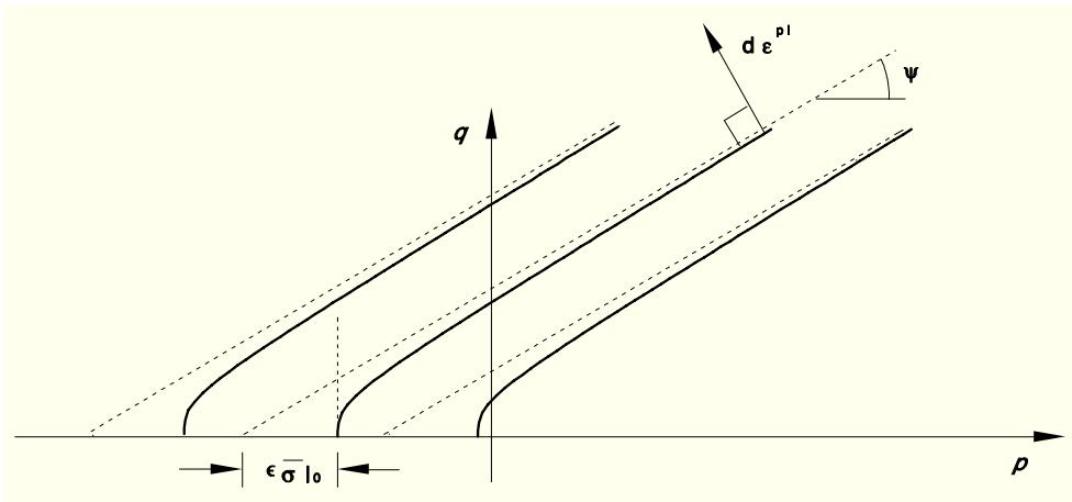
smooth, ensures that the flow direction is defined uniquely. The function asymptotically approaches the linear Drucker-Prager flow potential at high confining pressure stress and intersects the hydrostatic pressure axis at $9 0 ^ { \circ }$ . A family of hyperbolic potentials in the meridional stress plane is shown in Figure 4.4.2-6. The flow potential is a von Mises circle in the deviatoric stress plane (the ¦-plane). Figure 4.4.2-6 Family of hyperbolic flow potentials in the $p – q$ plane. 

text_image

dε^pl ψ q εσ l0 p

In both models flow is associated in the deviatoric stress plane. In the general exponent model, flow is always nonassociated in the meridional $p – q$ plane. In the hyperbolic model comparison of Equation 4.4.2-6 and Equation 4.4.2-9 shows that the flow is nonassociated in the $p – q$ plane if the dilation angle, Ã, and the material friction angle, $\beta ,$ are different. The hyperbolic model provides associated flow in the $p – q$ plane only when $\beta = \psi$ and $d ^ { \prime } \vert _ { 0 } /$ tan $\beta - p _ { t } | _ { 0 } = \epsilon \bar { \sigma } | _ { 0 }$ . # Creep models Classical "creep" behavior of materials that exhibit plastic behavior according to the extended Drucker-Prager models can be defined through the \*DRUCKER PRAGER CREEP option. The creep behavior in such materials is intimately tied to the plasticity behavior (through the definition of the creep flow potential and test data), so it is necessary to have the plasticity options \*DRUCKER PRAGER and \*DRUCKER PRAGER HARDENING present as part of the material behavior definition. The elastic part of the behavior must be linear. The rate-independent part of the plastic behavior is limited to the linear Drucker-Prager model with a von Mises (circular) section in the deviatoric stress plane ( K=1). The plastic potential is the hyperbolic flow potential described in conjunction with the hyperbolic and general exponent models (Equation 4.4.2-9). 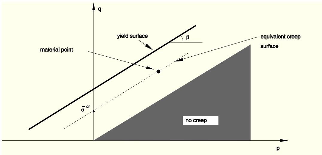# Creep behavior We adopt the notion of creep isosurfaces (or equivalent creep surfaces) of stress points that share the same creep "intensity," as measured by an equivalent creep stress. When the material plastifies, the equivalent creep surface should coincide with the yield surface; therefore, we define the equivalent creep surfaces by homogeneously scaling down the yield surface. In the $p – q$ plane that translates into parallels to the yield surface, as depicted in Figure 4.4.2-7. Figure 4.4.2-7 Equivalent creep stress defined as the shear stress. 

text_image

material point yield surface β equivalent creep surface σ⁻cr no creep p q

ABAQUS requires that creep properties be defined through the same type of test data used to define work hardening properties. The equivalent creep stress, $\bar { \boldsymbol { \sigma } } ^ { c r }$ , is determined as the intersection of the equivalent creep surface with the appropriate stress path. As a result, cr where $\beta ( \theta , f ^ { \alpha } )$ is the material angle of friction. Figure 4.4.2-7 shows how the equivalent creep stress is determined when the material properties are defined via a shear test: a parallel to the yield surface is drawn, such that it passes by the material point; the intersection of such a line with the test stress path $( p = 0 )$ produces $\bar { \boldsymbol { \sigma } } ^ { c r }$ . This approach has the consequence that the creep strain rate is a function of both q and p and allows realistic material properties to be determined in cases in which, due to high hydrostatic pressures, q is very high. If one looks at the yield strength of this material to be a composite of cohesion strength and friction strength, this model corresponds to cohesion-determined creep. Thus, there is a cone in p-q space inside which there is no creep. The built-in ABAQUS creep laws or the uniaxial laws defined through user subroutine CREEP can be used. The integration of the creep strain rate is first attempted explicitly, as described in \`\`Rate-dependent metal plasticity (creep),'' Section 4.3.4. If the stability limit is exceeded, a geometrically nonlinear analysis is being performed, or plasticity becomes active, the integration is done by the backward Euler method, as described in \`\`Rate-dependent metal plasticity (creep),'' Section 4.3.4. # Creep flow rule The creep flow rule is derived from a creep potential, $G ^ { c r }$ , in such a way that Equation 4.4.2-10 $$ d \varepsilon^ {c r} = \frac {d \bar {\varepsilon} ^ {c r}}{f ^ {c r}} \frac {\partial G ^ {c r}}{\partial \pmb {\sigma}}, $$ where $d \bar { \varepsilon } ^ { c r }$ is the equivalent creep strain rate, which must be work conjugate to the equivalent creep stress: $$ \begin{array}{l} d \bar {\varepsilon} ^ {c r} = | d \varepsilon_ {1 1} ^ {c r} | \quad \text {in the uniaxial compression case}, \\ = d \varepsilon_ {1 1} ^ {c r} \quad \text { in the uniaxial tension case }, \\ = \frac {d \gamma^ {c r}}{\sqrt {3}} \quad \mathrm{inthepureshearcase,where} \gamma^ {c r} \mathrm{istheengineeringshearcreepstrain.} \\ \end{array} $$ Since $d \pmb { \varepsilon } ^ { c r }$ is obviously work conjugate to ${ \pmb \sigma } , f ^ { c r }$ is defined by $$ f ^ {c r} = \frac {1}{\bar {\sigma} ^ {c r}} \pmb {\sigma}: \frac {\partial G ^ {c r}}{\partial \pmb {\sigma}}. $$ The equivalent creep strain rate is then determined from the "uniaxial" creep law: $$ d \bar {\varepsilon} ^ {c r} = h (\bar {\sigma} ^ {c r}, \bar {\varepsilon} ^ {c r}, \theta , f ^ {\alpha}). $$ The creep strain rate is assumed to follow from the same hyperbolic potential as the plastic strain rate Equation 4.4.2-11 $$ G ^ {c r} = \sqrt {(\epsilon \bar {\sigma} | _ {0} \tan \psi) ^ {2} + q ^ {2}} - p \tan \psi , $$ where $\psi ( \theta , f ^ { \alpha } )$ is the dilation angle measured in the p-q plane at high confining pressure; $\bar { \sigma } | _ { 0 } = \bar { \sigma } | _ { \bar { \varepsilon } ^ { p l } = 0 , \dot { \bar { \varepsilon } } ^ { p l } = 0 }$ is the initial yield stress; and ² is a parameter, referred to as the eccentricity, that defines the rate at which the function approaches the asymptote (the creep potential tends to a straight line as the eccentricity tends to zero). This creep potential, which is continuous and smooth, ensures that the creep flow direction is always uniquely defined. The function approaches the linear Drucker-Prager creep potential asymptotically at high confining pressure stress and intersects the hydrostatic pressure axis at 90°. A family of hyperbolic potentials in the meridional stress plane is shown in Figure 4.4.2-6. The creep potential is the von Mises circle in the deviatoric stress plane (the ¦-plane). Equation 4.4.2-10 and Equation 4.4.2-11 produce the complete flow rule $$ \Delta \varepsilon^ {c r} = \frac {\Delta \bar {\varepsilon} ^ {c r}}{f ^ {c r}} \bigg (\frac {q}{\sqrt {(\epsilon \bar {\sigma} | _ {0} \tan \psi) ^ {2} + q ^ {2}}} \mathbf {n} + \frac {1}{3} \tan \psi \mathbf {I} \bigg), $$ Equation 4.4.2-12 where $$ \mathbf {n} = \frac {\partial q}{\partial \pmb {\sigma}} = \frac {3}{2} \frac {\pmb {S}}{q}, $$ and $$ \begin{array}{l} f ^ {c r} = \frac {\bar {\sigma} ^ {c r}}{\sqrt {(\epsilon \bar {\sigma} _ {| 0} \tan \psi) ^ {2} + (\bar {\sigma} ^ {c r}) ^ {2}}} - \frac {1}{3} \tan \psi \quad \mathrm{ifcreepisdefinedviatheuniaxialcompressiondata,} \\ = \frac {\bar {\sigma} ^ {c r}}{\sqrt {(\epsilon \bar {\sigma} _ {| 0} \tan \psi) ^ {2} + (\bar {\sigma} ^ {c r}) ^ {2}}} + \frac {1}{3} \tan \psi \quad \mathrm{ifcreepisdefinedviatheuniaialtensiondata,} \\ = \frac {\bar {\sigma} ^ {c r}}{\sqrt {(\epsilon \bar {\sigma} _ {| 0} \tan \psi) ^ {2} + (\bar {\sigma} ^ {c r}) ^ {2}}} \quad \mathrm{ifcreepisdefinedvatheshardata}. \\ \end{array} $$ The expressions for $f ^ { c r }$ indicate that when creep properties are defined in terms of uniaxial compression data, $f ^ { c r }$ will become negative if $$ \bar {\sigma} ^ {c r} < \epsilon \bar {\sigma} _ {| 0} \frac {\frac {1}{3} (\tan \psi) ^ {2}}{\sqrt {1 - (\frac {1}{3} \tan \psi) ^ {2}}}. $$ Thus, below this stress level, which for typical materials will be very low, the stress vector and the normal to the creep potential are pointing in opposite directions: $$ \pmb {\sigma}: \frac {\partial G ^ {c r}}{\partial \pmb {\sigma}} < 0, $$ which is equivalent to $$ q - p \tan \psi < q - \frac {q ^ {2}}{\sqrt {(\epsilon \bar {\sigma} _ {| 0} \tan \psi) ^ {2} + q ^ {2}}}. $$ Therefore, if $\psi = \beta _ { \mathrm { i } }$ , there is a small zone just outside the "no creep" cone for which this is the case. Consequently, creep data obtained within this zone (such as data obtained in uniaxial compression) should show a creep strain rate in the opposite direction from the applied stress at very low stress levels, which will usually not be the case. To overcome this difficulty, ABAQUS will modify the creep data entered such that $f ^ { c r } \ge 0 . 1$ . Thus, one would not expect correspondence between calculated creep strains and measured creep properties in a region defined by $$ \bar {\sigma} ^ {c r} < \epsilon \bar {\sigma} _ {| 0} \frac {\alpha \tan \psi}{\sqrt {1 - \alpha^ {2}}}, $$ where $\alpha = 0 . 1 + \frac { 1 } { 3 } \tan \psi$ if the model is de¯ned in terms of uniaxial compression data ; $= 0 . 1 - \frac { 1 } { 3 } \tan \psi$ if the model is de¯ned in terms of uniaxial tension data ; = 0:1 if the model is de¯ned in terms of shear data : The exact size of this region depends on the value of tan à and the type of test data entered. This modification is usually not significant since typical creep analyses have loads that are applied quickly, followed by long-term creep. Hence, the stress level for most of the analysis will usually be well beyond the modified zone. An example of "slow" loading in which the approximation is visible is included in \`\`Verification of creep integration,'' Section 3.2.6 of the ABAQUS Benchmarks Manual. As is clear in the example, the effect of the approximation is small in spite of the fact that the load is ramped up over the step. Although creep flow is associated in the deviatoric stress plane, the use of a creep potential different from the equivalent creep surface implies that creep flow is nonassociated. # 4.4.3 Critical state models The inelastic constitutive theory provided in ABAQUS/Standard for modeling cohesionless materials is based on the critical state plasticity theory developed by Roscoe and his colleagues at Cambridge (Schofield et al., 1968, and Parry, 1972). The specific model implemented is an extension of the "modified Cam-clay" theory. The discussion is entirely in terms of effective stress: the soil may be saturated with a permeating fluid that carries a pressure stress and is assumed to flow according to Darcy's law. The continuum theory of this two phase material is described in \`\`Continuity statement for the wetting liquid phase in a porous medium,'' Section 2.8.4. The modified Cam-clay theory is a classical plasticity model. It uses a strain rate decomposition in which the rate of mechanical deformation of the soil is decomposed into an elastic and a plastic part; an elasticity theory; a yield surface; a flow rule; and a hardening rule. These various parts of the theory are defined in this section. The model is implemented numerically using backward Euler integration of the flow rule and hardening rule: this approach is used throughout ABAQUS for plasticity models. The basic ideas of the Cam-clay model are shown geometrically in Figure 4.4.3-1 to Figure 4.4.3-7. The main features of the model are the use of an elastic model (either linear elasticity or the porous elasticity model, which exhibits an increasing bulk elastic stiffness as the material undergoes compression) and for the inelastic part of the deformation a particular form of yield surface with associated flow and a hardening rule that allows the yield surface to grow or shrink. 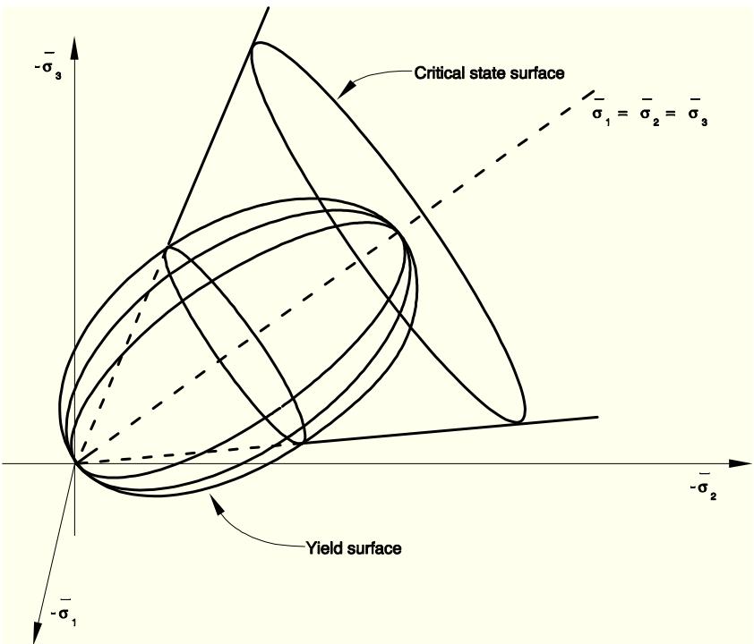A key feature of the model is the hardening/softening concept, which is developed around the introduction of a "critical state" surface: the locus of effective stress states where unrestricted, purely deviatoric, plastic flow of the soil skeleton occurs under constant effective stress. This critical state surface is assumed to be a cone in the space of principal effective stress ( Figure 4.4.3-1), whose vertex is the origin (zero effective stress) and whose axis is the equivalent pressure stress, p. Figure 4.4.3-1 Cam-clay yield and critical state surfaces in principal stress space. 

text_image

Critical state surface σ₁ = σ₂ = σ₃ Yield surface -σ₁ -σ₂ -σ₃

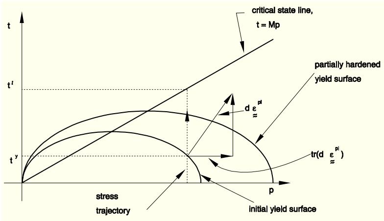
The section of the surface in the ¦-plane (the plane in principal stress space orthogonal to the equivalent pressure stress axis) is circular in the original form of the critical state model: in ABAQUS this has been extended to the more general shape shown in Figure 4.4.3-2. In the section of effective stress space defined by the equivalent pressure stress-- p--and a measure of equivalent deviatoric stress--t (the definition of t is given later in this section)--the critical state surface appears as a straight line, passing through the origin, with slope M (see Figure 4.4.3-2 and Figure 4.4.3-3). 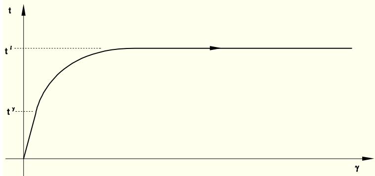Figure 4.4.3-2 Shear test response on the "dry" side of critical state $( t > M p )$ .  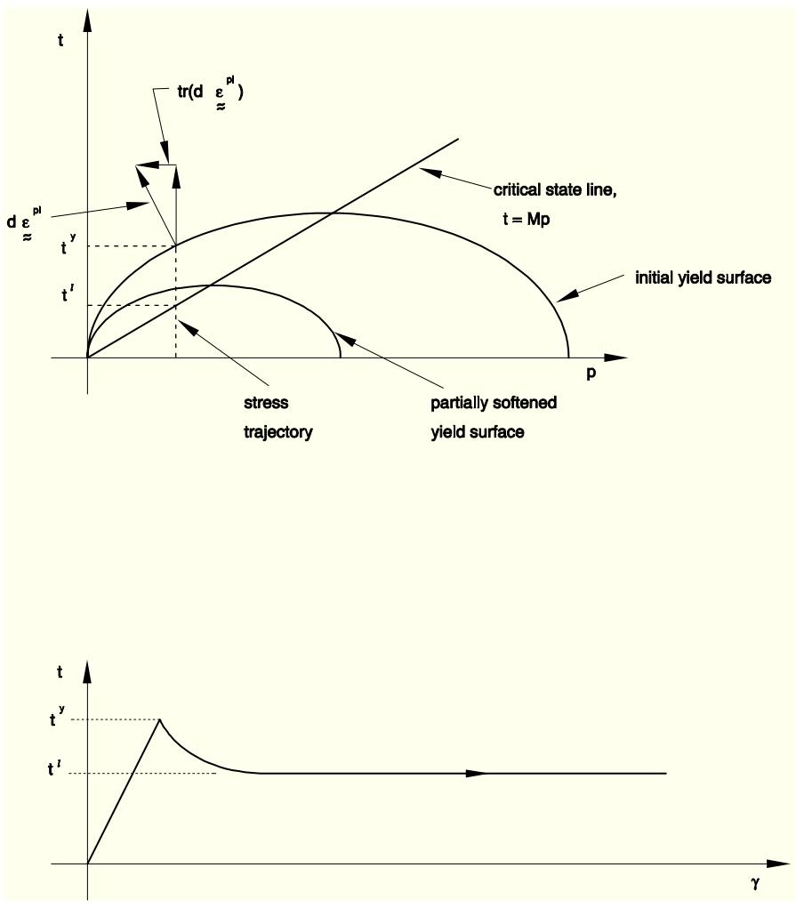Figure 4.4.3-3 Shear test response on the "wet" side of critical state ( t < M p). 

text_image

critical state line, t = Mp partially hardened yield surface d ε^pl tr(d ε^pl) t^y stress trajectory initial yield surface p


line

| γ | t | | ---- | ----- | | 0 | 0 | | >0 | t^y | | >0 | t^l |

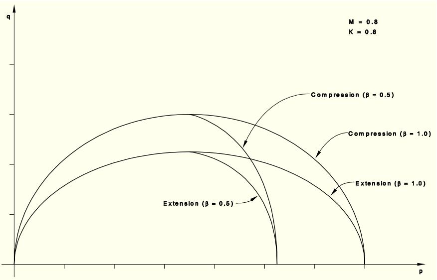
The modified Cam-clay yield surface has the same shape in the ¦-plane as the critical state surface, but in the $p { - } t$ plane it is assumed to be made up of two elliptic arcs: one arc passes through the origin with its tangent at right angles to the pressure stress axis and intersects the critical state line where its tangent is parallel to the pressure stress axis, while the other arc is a smooth continuation of the first arc through the critical state line and intersects the pressure stress axis at some nonzero value of pressure stress, again with its tangent at right angles to that axis (see Figure 4.4.3-4). Plastic flow is assumed to occur normal to this surface. Figure 4.4.3-4 Cam-clay yield surface in the $p – q$ plane. 

line

| p | q (Compression β = 0.5) | q (Compression β = 1.0) | q (Extension β = 0.5) | q (Extension β = 1.0) | |------|------------------------|------------------------|----------------------|----------------------| | Low | 0.0 | 0.0 | 0.0 | 0.0 | | Mid | ~0.8 | ~0.6 | ~0.7 | ~0.5 | | High | 0.0 | 0.0 | 0.0 | 0.0 |

The hardening/softening assumption controls the size of the yield surface in effective stress space. The hardening/softening is assumed to depend only on the volumetric plastic strain component and is such that, when the volumetric plastic strain is compressive (that is, when the soil skeleton is compacted), the yield surface grows in size, while inelastic increase in the volume of the soil skeleton causes the yield surface to shrink. The choice of elliptical arcs for the yield surface in the $( p , t )$ plane, together with the associated flow assumption, thus causes softening of the material for yielding states where $t > M p$ (to the left of the critical state line in Figure 4.4.3-2, the "dry" side of critical state) and hardening of the material for yielding states where $t < M p$ (to the right of the critical state line in Figure 4.4.3-3, the "wet" side of critical state). The resulting stress-strain behavior under states of constant effective pressure stress but increasing shear (deviatoric) strain is then as shown in Figure 4.4.3-2 and Figure 4.4.3-3: following initial yield (which is governed by the initially assumed yield surface size; that is, by the extent of initial overconsolidation) strain softening or strain hardening occurs until the stress state lies on the critical state surface when unrestricted deviatoric plastic flow (perfect plasticity) occurs. The terms "wet" and "dry" come from the idea of working a specimen of soil by hand. On the "wet" side of critical state the soil skeleton is too loosely compacted to support pressure stress--such stress, if applied (such as by squeezing the soil by hand) passes immediately into the pore water and thus causes this water to bleed out of the specimen and wet the hands. The opposite effect occurs when the soil is on the "dry" side of critical state. The preceding discussion describes the concepts of the theory. These are now formalized, as they are implemented in ABAQUS/Standard. # The strain rate decomposition The volume change is decomposed as Equation 4.4.3-1 $$ J = J ^ {g} \cdot J ^ {e l} \cdot J ^ {p l}, $$ where J is the ratio of current volume to original volume, $J ^ { g }$ is the ratio of current to original volume of the soil grain particles, $J ^ { e l }$ is the elastic (recoverable) part of the ratio of current to original volume of the soil volume, and $J ^ { p l }$ is the plastic (nonrecoverable) part of the ratio of current to original volume of the soil volume. Volumetric strains are defined as $$ \varepsilon_ {\mathrm{vol}} = \ln J, $$ $$ \varepsilon_ {\mathrm{vol}} ^ {e l} = \ln J ^ {e l}, $$ $$ \varepsilon_ {\mathrm{vol}} ^ {p l} = \ln J ^ {p l}. $$ These definitions and Equation 4.4.3-1 result in the usual additive strain rate decomposition for volumetric strain rates: Equation 4.4.3-2 $$ d \varepsilon_ {\mathrm{vol}} = d \varepsilon_ {\mathrm{vol}} ^ {g} + d \varepsilon_ {\mathrm{vol}} ^ {e l} + d \varepsilon_ {\mathrm{vol}} ^ {p l}. $$ The model also assumes the deviatoric strain rates decompose in an additive manner, so that the total strain rates decompose as $$ d \pmb {\varepsilon} = d \varepsilon_ {\mathrm{vol}} ^ {g} \mathbf {I} + d \pmb {\varepsilon} ^ {e l} + d \pmb {\varepsilon} ^ {p l}, $$ where I is a unit matrix. # Elastic behavior The elastic behavior can be modeled as linear or by using the porous elasticity model, typically with a zero tensile strength, as described in \`\`Porous elasticity,'' Section 4.4.1. # Plastic behavior The modified Cam-clay yield function is defined in terms of the equivalent effective pressure stress, p, and the Mises equivalent stress and third stress invariant, defined as $$ p = - \frac {1}{3} \mathrm{trace} \pmb {\sigma} = - \frac {1}{3} \pmb {\sigma}: \mathbf {I} $$ $$ q = \sqrt {\frac {3}{2} \mathbf {S} : \mathbf {S}} $$ $$ r ^ {3} = \frac {9}{2} \mathbf {S}: \mathbf {S} \cdot \mathbf {S}. $$ The surface is Equation 4.4.3-3 $$ f (p, q, r) = \frac {1}{\beta^ {2}} \left(\frac {p}{a} - 1\right) ^ {2} + \left(\frac {t}{M a}\right) ^ {2} - 1 = 0. $$