```csv 90 DUM=1./XBAR K2=0 DO 100 K=1,4 K2=K2 + 2 B(4,K2 ) = 0. 100 B(4,K2-1) = H(K)*DUM GO TO 900 C 800 STOP 900 RETURN C 2000 FORMAT (//,' *** ERROR *** ', 1 ' ZERO OR NEGATIVE JACOBIAN DETERMINANT FOR ELEMENT ( ',I8,' )')QUA00246 C END QUA00234 QUA00235 QUA00236 QUA00237 QUA00238 QUA00239 QUA00240 QUA00241 QUA00242 QUA00243 QUA00244 QUA00245 QUA00246 QUA00247 QUA00248 ``` # Finite Element Nonlinear Analysis in Solid and Structural Mechanics # 6.1 INTRODUCTION TO NONLINEAR ANALYSIS In the finite element formulation given in Section 4.2, we assumed that the displacements of the finite element assemblage are infinitesimally small and that the material is linearly elastic. In addition, we also assumed that the nature of the boundary conditions remains unchanged during the application of the loads on the finite element assemblage. With these assumptions, the finite element equilibrium equations derived were for static analysis $$ \mathbf {K U} = \mathbf {R} \tag {6.1} $$ These equations correspond to a linear analysis of a structural problem because the displacement response U is a linear function of the applied load vector R; i.e., if the loads are $\alpha R$ instead of R, where $\alpha$ is a constant, the corresponding displacements are $\alpha U$ . When this is not the case, we perform a nonlinear analysis. The linearity of a response prediction rests on the assumptions just stated, and it is instructive to identify in detail where these assumptions have entered the equilibrium equations in (6.1). The fact that the displacements must be small has entered into the evaluation of the matrix K and load vector R because all integrations have been performed over the original volume of the finite elements, and the strain-displacement matrix B of each element was assumed to be constant and independent of the element displacements. The assumption of a linear elastic material is implied in the use of a constant stress-strain matrix C, and, finally, the assumption that the boundary conditions remain unchanged is reflected in the use of constant constraint relations [see (4.43) to (4.46)] for the complete response. If during loading a displacement boundary condition should change, e.g., a degree of freedom which was free becomes restrained at a certain load level, the response is linear only prior to the change in boundary condition. This situation arises, for example, in the analysis of a contact problem (see Example 6.2 and Section 6.7). The above discussion of the basic assumptions used in a linear analysis defines what we mean by a nonlinear analysis and also suggests how to categorize different nonlinear analyses. Table 6.1 gives a classification that is used conveniently because it considers separately material nonlinear effects and kinematic nonlinear effects. The formulations listed in the table are those that we shall discuss in this chapter. TABLE 6.1 Classification of nonlinear analyses

Type of analysis	Description	Typical formulation used	Stress and strain measures
Materially-nonlinear-only	Infinitesimal displacements and strains; the stress-strain relation is nonlinear	Materially-nonlinear-only (MNO)	Engineering stress and strain
Large displacements, large rotations, but small strains	Displacements and rotations of fibers are large, but fiber extensions and angle changes between fibers are small; the stress-strain relation may be linear or nonlinear	Total Lagrangian (TL)	Second Piola-Kirchhoff stress, Green-Lagrange strain
		Updated Lagrangian (UL)	Cauchy stress, Almansi strain
Large displacements, large rotations, and large strains	Fiber extensions and angle changes between fibers are large, fiber displacements and rotations may also be large; the stress-strain relation may be linear or nonlinear	Total Lagrangian (TL)	Second Piola-Kirchhoff stress, Green-Lagrange strain
		Updated Lagrangian (UL)	Cauchy stress, logarithmic strain

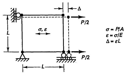
Figure 6.1 gives an illustration of the types of problems that are encountered, as listed in Table 6.1. We should note that in a materially-nonlinear-only analysis, the nonlinear effect lies only in the nonlinear stress-strain relation. The displacements and strains are infinitesimally small; therefore the usual engineering stress and strain measures can be employed in the response description. Considering the large displacement but small strain conditions, we note that in essence the material is subjected to infinitesimally small strains measured in a body-attached coordinate frame $x'$ , $y'$ while this frame undergoes large rigid body displacements and rotations. The stress-strain relation of the material can be linear or nonlinear. As shown in Fig. 6.1 and Table 6.1, the most general analysis case is the one in which the material is subjected to large displacements and large strains. In this case the stress-strain relation is also usually nonlinear. In addition to the analysis categories listed in Table 6.1, Fig. 6.1 illustrates another type of nonlinear analysis, namely, the analysis of problems in which the boundary conditions change during the motion of the body under consideration. This situation arises in 

text_image

L σ, ε P/2 P/2 L Δ σ = P/A ε = σ/E Δ = εL


text_image

σ E 1 ε ε < 0.02

(a) Linear elastic (infinitesimal displacements) 

text_image

L P/2 Δ P/2 L σ = P/A ε = σY/E + σ - σY/ET ε < 0.02


line

| ε | σ | Label | | ---- | ---- | ----- | | 1 | 0 | E | | 1 | 1 | E_T | | 1 | 1 | P/A |

(b) Materially-nonlinear-only (infinitesimal displacements, but nonlinear stress-strain relation) 

text_image

y L x y' Δ' ε' L x' ε' < 0.02 Δ' = ε'L

(c) Large displacements and large rotations but small strains. Linear or nonlinear material behavior Figure 6.1 Classification of analyses 

flowchart

```mermaid graph TD A["Square"] --> B["Pentagon"] ```

(d) Large displacements, large rotations, and large strains. Linear or nonlinear material behavior 

text_image

P/2 A P/2 Δ

(e) Change in boundary condition at displacement $\Delta$ Figure 6.1 (continued) particular in the analysis of contact problems, of which a simple example is given in Fig. 6.1(e). In general, this change in boundary condition may be encountered in any one of the analyses summarized in Table 6.1. In actual analysis, it is necessary to decide whether a problem falls into one or the other category of analysis, and this dictates which formulation will be used to describe the actual physical situation. Conversely, we may say that by the use of a specific formulation, a model of the actual physical situation is assumed, and the choice of formulation is part of the complete modeling process. Surely, the use of the most general large strain formulation "will always be correct"; however, the use of a more restrictive formulation may be computationally more effective and may also provide more insight into the response prediction. Before we discuss the general formulations of nonlinear analyses, it would be instructive to consider first two simple examples that demonstrate some of the features listed in Table 6.1. EXAMPLE 6.1: A bar rigidly supported at both ends is subjected to an axial load as shown in Fig. E6.1(a). The stress-strain relation and the load-versus-time curve relation are given in Figs. E6.1(b) and (c), respectively. Assuming that the displacements and strains are small and that the load is applied slowly, calculate the displacement at the point of load application. 

text_image

Area A = 1 cm² tU tR Section a Section b Lb = 10 cm Lb = 5 cm

(a) Simple bar structure 

line

| ε | σ | Label | |-------|-------|-----------| | 0.002 | 1 | E | | 0.002 | 1 | E_T | | 0.002 | 1 | E_T |

(b) Stress-strain relation (in tension and compression) 

line

| Time (sec) | tR (×10⁴ N) | | ---------- | ----------- | | 0 | 0 | | 2 | 4 | | 3 | 1.5 | | 7 | 1.5 |

(c) Load variation Figure E6.1 Analysis of simple bar structure Since the load is applied slowly and the displacements and strains are small, we calculate the response of the bar using a static analysis with material nonlinearities only. Then we have for sections a and b, the strain relations $$ ^ \prime \epsilon_ {a} = \frac {^ \prime u}{L _ {a}}; \quad \quad^ {\prime} \epsilon_ {b} = - \frac {^ \prime u}{L _ {b}} \tag {a} $$ the equilibrium relations, $$ ^ \prime R + ^ {\prime} \sigma_ {b} A = ^ {\prime} \sigma_ {a} A \tag {b} $$ and the constitutive relations, under loading conditions, $$ \begin{array}{l} ^ \prime \epsilon = \frac {^ \prime \sigma}{E} \quad \text { in the elastic region } \\ ^ t \epsilon = \epsilon_ {y} + \frac {^ t \sigma - \sigma_ {y}}{E _ {T}} \quad \text { in the plastic region } \\ \end{array} $$ (c) and in unloading, $$ \Delta \epsilon = \frac {\Delta \sigma}{E} $$ In these relations the superscript t denotes “at time t.” (i) Both sections $a$ and $b$ are elastic During the initial phase of load application both sections $a$ and $b$ are elastic. Then we have, using (a) to (c), $$ ^ \prime R = E A ^ {\prime} u \left(\frac {1}{L _ {a}} + \frac {1}{L _ {b}}\right) $$ and substituting the values given in Fig. E6.1, we obtain $$ ^ \prime u = \frac {^ \prime R}{3 \times 1 0 ^ {6}} $$ with $^{t}\sigma_{a}=\frac{^{\prime}R}{3A};\quad^{t}\sigma_{b}=-\frac{2}{3}\frac{^{\prime}R}{A}$ (d) (ii) Section $a$ is elastic while section $b$ is plastic Section b will become plastic at time $t^{*}$ when, using (d), $$ ^ {r ^ {*}} R = \frac {3}{2} \sigma_ {y} A $$ Afterward we therefore have $$ { } ^ { t } \sigma _ { a } = E \frac { { } ^ { t } u } { L _ { a } } \tag {e} $$ $$ ^ t \sigma_ {b} = - E _ {T} \left(\frac {^ t u}{L _ {b}} - \epsilon_ {y}\right) - \sigma_ {y} $$ Using (e), we therefore have for $t \geq t^*$ , $$ ^ t R = \frac {E A ^ {t} u}{L _ {a}} + \frac {E _ {T} A ^ {t} u}{L _ {b}} - E _ {T} \epsilon_ {y} A + \sigma_ {y} A $$ and thus $^t u = \frac{^t R / A + E_T \epsilon_y - \sigma_y}{(E / L_a) + (E_T / L_b)}$ $$ = \frac {^ \prime R}{1 . 0 2 \times 1 0 ^ {6}} - 1. 9 4 1 2 \times 1 0 ^ {- 2} $$ We may note that section $a$ would become plastic when $^t\sigma_a = \sigma_y$ or $^t R = 4.02 \times 10^4$ N. Since the load does not reach this value [see Fig. E6.1(c)], section $a$ remains elastic throughout the response history. (iii) In unloading both sections act elastically we have $\Delta u = \frac{\Delta R}{EA[(1 / L_a) + (1 / L_b)]}$ The calculated response is depicted in Fig. E6.1(d). 

line

| t_u (cm) | t_R (×10⁴ N) | | -------- | ------------ | | 0.005 | 0.0 | | 0.01 | 1.5 | | 0.015 | 3.0 | | 0.02 | 4.0 |

(d) Calculated response Figure E6.1 (continued) EXAMPLE 6.2: A pretensioned cable is subjected to a transverse load midway between the supports as shown in Fig. E6.2(a). A spring is placed below the load at a distance $w_{gap}$ . Assume that the displacements are small so that the force in the cable remains constant, and that the load is applied slowly. Calculate the displacement under the load as a function of the load intensity. 

text_image

L = 100 cm tR L = 100 cm tw wgap = 1 cm Tension H = 100 N Spring constant k = 2 N/cm

(a) Pretensioned cable subjected to transverse load 

text_image

R (N) 1 1 Time

(b) Load 

line

| r_w (cm) | r (N) | |---|---| | 0 | 0 | | 1 | 2 | | 2 | 6 |

(c) Calculated response Figure E6.2 Analysis of pretensioned cable with a spring support As in Example 6.1, we neglect inertia forces and assume small displacements. As long as the displacement 'w under the load is smaller than $w_{gap}$ , vertical equilibrium requires for small 'w, $$ ^ \prime R = 2 H \frac {^ \prime w}{L} \tag {a} $$ Once the displacement is larger than $w_{gap}$ , the following equilibrium equation holds: $$ ^ \prime R = 2 H \frac {^ \prime w}{L} + k (^ {\prime} w - w _ {\text { gap }}) \tag {b} $$ Figure E6.2(c) shows graphically the force displacement relations given in (a) and (b). We should note that in this analysis we neglected the elasticity of the cable; therefore the response is calculated using only the equilibrium equations in (a) and (b), and the only nonlinearity is due to the contact condition established when $w \geq w_{\text{gap}}$ . Although these examples represent two very simple problems, the given solutions display some important general features. The basic problem in a general nonlinear analysis is to find the state of equilibrium of a body corresponding to the applied loads. Assuming that the externally applied loads are described as a function of time, as in Examples 6.1 and 6.2, the equilibrium conditions of a system of finite elements representing the body under consideration can be expressed as $$ ^ \prime \mathbf {R} - ^ {\prime} \mathbf {F} = \mathbf {0} \tag {6.2} $$ where the vector 'R lists the externally applied nodal point forces in the configuration at time t and the vector 'F lists the nodal point forces that correspond to the element stresses in this configuration. Hence, using the notation in Chapter 4, relations (4.18) and (4.20) to (4.22), we have $$ ^ \prime \mathbf {R} = ^ {\prime} \mathbf {R} _ {B} + ^ {\prime} \mathbf {R} _ {S} + ^ {\prime} \mathbf {R} _ {C} \tag {6.3} $$ and, identifying the current stresses as initial stresses, $R_{I} = {}^{t}F$ , $$ { } ^ { t } \mathbf { F } = \sum _ { m } \int _ { t _ { V ( m ) } } { } ^ { t } \mathbf { B } ^ { ( m ) T } { } ^ { t } \boldsymbol { \tau } ^ { ( m ) } { } ^ { t } d V ^ { ( m ) } \tag {6.4} $$ where in a general large deformation analysis the stresses as well as the volume of the body at time t are unknown. The relation in (6.2) must express the equilibrium of the system in the current deformed geometry taking due account of all nonlinearities. Also, in a dynamic analysis, the vector 'R would include the inertia and damping forces, as discussed in Section 4.2.1. Considering the solution of the nonlinear response, we recognize that the equilibrium relation in $(6.2)$ must be satisfied throughout the complete history of load application; i.e., the time variable t may take on any value from zero to the maximum time of interest (see Examples 6.1 and 6.2). In a static analysis without time effects other than the definition of the load level (e.g., without creep effects; see Section 6.6.3), time is only a convenient variable which denotes different intensities of load applications and correspondingly different configurations. However, in a dynamic analysis and in static analysis with material time effects, the time variable is an actual variable to be properly included in the modeling of the actual physical situation. Based on these considerations, we realize that the use of the time variable to describe the load application and history of solution represents a very general approach and corresponds to our earlier assertion that a “dynamic analysis is basically a static analysis including inertia effects.” As for the analysis results to be calculated, in many solutions only the stresses and displacements reached at specific load levels or at specific times are required. In some nonlinear static analyses the equilibrium configurations corresponding to these load levels can be calculated without also solving for other equilibrium configurations. However, when the analysis includes path-dependent nonlinear geometric or material conditions, or time-dependent phenomena, the equilibrium relations in (6.2) need to be solved for the complete time range of interest. This response calculation is effectively carried out using a step-by-step incremental solution, which reduces to a one-step analysis if in a static time-independent solution the total load is applied all together and only the configuration corresponding to that load is calculated. However, we shall see that for computational reasons, in practice, even the analysis of such a case frequently requires an incremental solution, performed automatically (see also Section 8.4), with a number of load steps to finally reach the total applied load. The basic approach in an incremental step-by-step solution is to assume that the solution for the discrete time t is known and that the solution for the discrete time $t + \Delta t$ is required, where $\Delta t$ is a suitably chosen time increment. Hence, considering (6.2) at time $t + \Delta t$ we have $$ { } ^ { t + \Delta t } \mathbf { R } - { } ^ { t + \Delta t } \mathbf { F } = \mathbf { 0 } \tag {6.5} $$ where the left superscript denotes “at time $t + \Delta t$ .” Assume that $t^{+ \Delta t} R$ is independent of the deformations. Since the solution is known at time t, we can write $$ ^ {t + \Delta t} \mathbf {F} = ^ {t} \mathbf {F} + \mathbf {F} \tag {6.6} $$ where F is the increment in nodal point forces corresponding to the increment in element displacements and stresses from time t to time $t + \Delta t$ . This vector can be approximated using a tangent stiffness matrix 'K which corresponds to the geometric and material conditions at time t, $$ \mathbf {F} \doteq {} ^ {\prime} \mathbf {K U} \tag {6.7} $$ where U is a vector of incremental nodal point displacements and $$ ^ \prime \mathbf {K} = \frac {\partial^ {\prime} \mathbf {F}}{\partial^ {\prime} \mathbf {U}} \tag {6.8} $$ Hence, the tangent stiffness matrix corresponds to the derivative of the internal element nodal point forces 'F with respect to the nodal point displacements 'U. Substituting (6.7) and (6.6) into (6.5), we obtain $$ ^ t \mathbf {K} \mathbf {U} = ^ {t + \Delta t} \mathbf {R} - ^ {t} \mathbf {F} \tag {6.9} $$ and solving for U, we can calculate an approximation to the displacements at time $t + \Delta t$ , $$ ^ {t + \Delta t} \mathbf {U} \doteq {} ^ {t} \mathbf {U} + \mathbf {U} \tag {6.10} $$ The exact displacements at time $t + \Delta t$ are those that correspond to the applied loads $t^{+}\Delta t^{r}R$ . We calculate in (6.10) only an approximation to these displacements because (6.7) was used. Much of our discussion in this chapter will focus on the proper and effective evaluation of 'F and 'K. Having evaluated an approximation to the displacements corresponding to time $t + \Delta t$ , we could now solve for an approximation to the stresses and corresponding nodal point forces at time $t + \Delta t$ , and then proceed to the next time increment calculations. However, because of the assumption in (6.7), such a solution may be subject to very significant errors and, depending on the time or load step sizes used, may indeed be unstable. In practice, it is therefore necessary to iterate until the solution of (6.5) is obtained to sufficient accuracy. The widely used iteration methods in finite element analysis are based on the classical Newton-Raphson technique (see, for example, E. Kreyszig [A] and see N. Bićanić and K. H. Johnson [A]), which we formally derive in Section 8.4. This method is an extension of the simple incremental technique given in (6.9) and (6.10). That is, having calculated an increment in the nodal point displacements, which defines a new total displacement vector, we can repeat the incremental solution presented above using the currently known total displacements instead of the displacements at time t. The equations used in the Newton-Raphson iteration are, for $i = 1, 2, 3, \ldots$ , $$ \begin{array}{l} { } ^ { t + \Delta t } \mathbf { K } ^ { ( i - 1 ) } \Delta \mathbf { U } ^ { ( i ) } = { } ^ { t + \Delta t } \mathbf { R } - { } ^ { t + \Delta t } \mathbf { F } ^ { ( i - 1 ) } \tag {6.11} \\ { } ^ { t + \Delta t } \mathbf { U } ^ { ( i ) } = { } ^ { t + \Delta t } \mathbf { U } ^ { ( i - 1 ) } + \Delta \mathbf { U } ^ { ( i ) } \\ \end{array} $$ with the initial conditions $$ { } ^ { t + \Delta t } \mathbf { U } ^ { ( 0 ) } = { } ^ { t } \mathbf { U } ; \quad { } ^ { t + \Delta t } \mathbf { K } ^ { ( 0 ) } = { } ^ { t } \mathbf { K } ; \quad { } ^ { t + \Delta t } \mathbf { F } ^ { ( 0 ) } = { } ^ { t } \mathbf { F } \tag {6.12} $$ Note that in the first iteration, the relations in (6.11) reduce to the equations (6.9) and (6.10). Then, in subsequent iterations, the latest estimates for the nodal point displacements