# 1. Equation of motion $$ \int_ {0 _ {V}} ^ {t + \Delta_ {0} ^ {t}} S _ {i j} \delta^ {t + \Delta_ {0} ^ {t}} \epsilon_ {i j} d ^ {0} V = ^ {t + \Delta_ {t}} \mathcal {R} $$ where $$ { } ^ { t + \Delta t } { } _ { 0 } S _ { i j } = \frac { { } ^ { 0 } \rho } { { } ^ { t + \Delta t } \rho } { } ^ { t + \Delta t } x _ { i , m } { } ^ { t + \Delta t } { } _ { T _ { m n } } { } ^ { t + \Delta t } { } _ { t + \Delta t } ^ { 0 } x _ { j , n } ; \qquad \delta ^ { t + \Delta t } { } _ { 0 } \epsilon _ { i j } = \delta \frac { 1 } { 2 } \left( { } ^ { t + \Delta t } { } _ { 0 } u _ { i , j } + { } ^ { t + \Delta t } { } _ { 0 } u _ { j , i } + { } ^ { t + \Delta t } { } _ { 0 } u _ { k , i } { } ^ { t + \Delta t } { } _ { 0 } u _ { k , j } \right) $$ # 2. Incremental decompositions (a) Stresses $$ ^ {i + \Delta_ {0} ^ {i}} S _ {i j} = _ {0} ^ {i} S _ {i j} + _ {0} S _ {i j} $$ (b) Strains $$ \begin{array}{l} { } ^ { \prime + \Delta } \epsilon _ { i j } = \epsilon _ { i j } + _ { 0 } \epsilon _ { i j } ; \quad \quad _ { 0 } \epsilon _ { i j } = _ { 0 } e _ { i j } + _ { 0 } \eta _ { i j } \\ _ 0 e _ {i j} = \frac {1}{2} (_ {0} u _ {i, j} + _ {0} u _ {j, i} + _ {0} u u _ {k, j} + _ {0} u u _ {k, j}); \quad_ {0} \eta_ {i j} = \frac {1}{2} _ {0} u u _ {k, j} \\ \end{array} $$ Initial displacement effect # 3. Equation of motion with incremental decompositions Noting that $\delta^{+}\Delta_{0}^{\prime}\epsilon_{ij} = \delta_{0}\epsilon_{ij}$ the equation of motion is $$ \int S _ {i j} \delta_ {0} \epsilon_ {i j} d ^ {0} V + \int ^ {t} S _ {i j} \delta_ {0} \eta_ {i j} d ^ {0} V = ^ {t + \Delta t} \mathcal {R} - \int ^ {t} S _ {i j} \delta_ {0} e _ {i j} d ^ {0} V $$ # 4. Linearization of equation of motion Using the approximations $_0S_{ij} = _0C_{ijrs}$ $_0e_{rs}$ , $\delta_0\epsilon_{ij} = \delta_0e_{ij}$ , we obtain as approximate equation of motion: $$ \int C _ {i j r s 0} e _ {r s} \delta_ {0} e _ {i j} d ^ {0} V + \int ^ {i} S _ {i j} \delta_ {0} \eta_ {i j} d ^ {0} V = ^ {i + \Delta \kappa} \mathcal {R} - \int ^ {i} S _ {i j} \delta_ {0} e _ {i j} d ^ {0} V $$ # TABLE 6.3 Continuum mechanics incremental decomposition: Updated Lagrangian formulation # 1. Equation of motion $$ \int_ {t _ {V}} ^ {t + \Delta t} S _ {i j} \delta^ {t + \Delta t} \epsilon_ {i j} d ^ {t} V = ^ {t + \Delta t} \mathcal {R} $$ where $$ { } ^ { t + \Delta t } S _ { i j } = \frac { { } ^ { t } \rho } { { } ^ { t + \Delta t } \rho } { } ^ { t + \Delta t } x _ { i , m } { } ^ { t + \Delta t } \tau _ { m n } { } ^ { t + \Delta t } x _ { j , n } ; \quad \delta ^ { t + \Delta t } \epsilon _ { i j } = \delta \frac { 1 } { 2 } ( { } _ { t } u _ { i , j } + { } _ { t } u _ { j , i } + { } _ { t } u _ { k , i } { } _ { t } u _ { k , j } ) $$ # 2. Incremental decompositions (a) Stresses $$ ^ {r + \Delta_ {i}} S _ {i j} = ^ {r} \tau_ {i j} + _ {r} S _ {i j} \quad \text { note that } ^ {i} S _ {i j} \equiv^ {r} \tau_ {i j} $$ (b) Strains $$ { } ^ { t + \Delta } { } _ { t } \epsilon _ { i j } = { } _ { t } \epsilon _ { i j } ; \quad \epsilon _ { i j } = { } _ { t } e _ { i j } + { } _ { t } \eta _ { i j } $$ $$ _ {i} e _ {i j} = \frac {1}{2} (_ {i} u _ {i, j} + _ {i} u _ {j, i}); \quad \eta_ {i j} = \frac {1}{2} _ {i} u u _ {k, j} $$ # 3. Equation of motion with incremental decompositions The equation of motion is $$ \int_ {t _ {V}} ^ {t} S _ {i j} \delta_ {t} \epsilon_ {i j} d ^ {t} V + \int_ {t _ {V}} ^ {t} \tau_ {i j} \delta_ {t} \eta_ {i j} d ^ {t} V = ^ {t + \Delta t} \mathcal {R} - \int_ {t _ {V}} ^ {t} \tau_ {i j} \delta_ {t} e _ {i j} d ^ {t} V $$ # 4. Linearization of equation of motion Using the approximations $_{t}S_{ij} = _{t}C_{ijrs} e_{rs}$ , $\delta_{t}\epsilon_{ij} = \delta_{t}e_{ij}$ , we obtain as approximate equation of motion: $$ \int_ {t _ {V}} ^ {t} C _ {i j r s} e _ {r s} \delta_ {t} e _ {i j} d ^ {\prime} V + \int_ {t _ {V}} ^ {t} \tau_ {i j} \delta_ {t} \eta_ {i j} d ^ {\prime} V = ^ {t + \Delta t} \mathcal {R} - \int_ {t _ {V}} ^ {t} \tau_ {i j} \delta_ {t} e _ {i j} d ^ {\prime} V $$ where $_{0}C_{ijrs}$ and $_{t}C_{ijrs}$ are the incremental stress-strain tensors at time t referred to the configurations at times 0 and t, respectively. The derivation of $_{0}C_{ijrs}$ and $_{t}C_{ijrs}$ for various materials is discussed in Section 6.6. We also note that in (6.74) and (6.75) $_{0}S_{ij}$ and $_{t}\tau_{ij}$ are the known second Piola-Kirchhoff and Cauchy stresses at time t; and $_{0}e_{ij}$ , $_{0}\eta_{ij}$ and $_{t}e_{ij}$ , $_{t}\eta_{ij}$ are the linear and nonlinear incremental strains which are referred to the configurations at times 0 and t, respectively. Let us consider in more detail the steps performed in Table 6.2. The steps in Table 6.3 are performed analogously. In step 2, we incrementally decompose the stresses and strains, which is allowed because all stresses and strains, including the increments, are referred to the original (same) configuration. Also note that we obtain the incremental Green-Lagrange strain components in Table 6.2 by simply using $_{0}\epsilon_{ij} = ^{t+\Delta t}_{0}\epsilon_{ij} - _{0}^{\prime}\epsilon_{ij}$ and expressing $^{t+\Delta t}_{0}\epsilon_{ij}$ and $_{0}^{\prime}\epsilon_{ij}$ in terms of the displacements, where $^{t+\Delta t}_{i}u_{i} = ^{t}u_{i} + u_{i}$ . In step 3, we use $\delta^{t + \Delta t}_{0}\epsilon_{ij} = \delta ({}_{0}^{\prime}\epsilon_{ij} + {}_{0}\epsilon_{ij}) = \delta_{0}\epsilon_{ij}$ ; that is, here $\delta_0^\prime \epsilon_{ij} = 0$ because the variation is taken about the configuration at time $t + \Delta t$ . We also bring all known quantities to the right-hand side in the principle of virtual work equation. Note that for a given displacement variation the expression $\int_{0V}{}_{0}^{\prime}S_{ij}\delta_{0}e_{ij}d^{0}V$ is known. So far we have not made any assumption but have merely rewritten the original principle of virtual work equation. In general, the left-hand side of the principle of virtual work equation given in step 3 is highly nonlinear in the incremental displacements $u_{i}$ . In step 4, we now linearize the expression, and this linearization is achieved in the following manner. First, we note that the term $\int_{0V} \delta_S \delta_0 \eta_{ij} d^0 V$ is already linear in the incremental displacements; hence, we keep this term without change. The nonlinear effects are due to the term $\int_{0V} S_{ij} \delta_0 \epsilon_{ij} d^0 V$ , which we linearize using a Taylor series expansion, $$ \begin{array}{l} \int S _ {i j} \delta_ {0} \epsilon_ {i j} d ^ {0} V = \int_ {0 _ {V}} \left( \right.\frac {\partial_ {0} ^ {\prime} S _ {i j}}{\partial_ {0} ^ {\prime} \epsilon_ {r s}} \left. \right| \epsilon_ {r s} + \text { higher order terms } \left) \delta_ {(0} e _ {i j} + _ {0} \eta_ {i j}\left. \right) d ^ {0} V \\ = \int_ {0 _ {V}} \left( \right.\underbrace {\frac {\partial_ {0} ^ {t} S _ {i j}}{\partial_ {0} ^ {t} \epsilon_ {r s} \mid_ {t}}} _ {0 C _ {i j r s}} \left(_ {0} e _ {r s} + \underbrace {_ {0} \eta_ {r s}} _ {\text {Neglect}} + \underbrace {\text {higher order terms}} _ {\text {Neglect}}\right) \delta_ {\left(_ {0} e _ {i j} + \underbrace {_ {0} \eta_ {i j}} _ {\text {Neglect}}\right)} d ^ {0} V \\ \doteq \int C e _ {r s} \delta_ {0} e _ {i j} d ^ {0} V \\ \end{array} $$ This term is now linear in the incremental displacements because $\delta_0e_{ij}$ is independent of the $u_{i}$ . Comparing the UL and TL formulations in Tables 6.2 and 6.3, we observe that they are quite analogous and that, in fact, the only theoretical difference between the two formulations lies in the choice of different reference configurations for the kinematic and static variables. Indeed, if in the numerical solution the appropriate constitutive tensors are employed, identical results are obtained (see Section 6.6). The choice of using either the UL or the TL formulation in a finite element solution depends, in practice, on their relative numerical effectiveness, which in turn depends on the finite element and the constitutive law used. However, one general observation can be made considering Tables 6.2 and 6.3, namely, that the incremental linear strains $_{0}e_{ij}$ in the TL formulation contain an initial displacement effect that leads to a more complex strain-displacement matrix than in the UL formulation. The relations in (6.74) and (6.75) can be employed to calculate an increment in the displacements, which then is used to evaluate approximations to the displacements, strains, and stresses corresponding to time $t + \Delta t$ . The displacement approximations corresponding to $t + \Delta t$ are obtained simply by adding the calculated increments to the displacements at time t, and the strain approximations are evaluated from the displacements using the available kinematic relations [e.g., relation (6.54) in the TL formulation]. However, the evaluation of the stresses corresponding to time $t + \Delta t$ depends on the specific constitutive relations used and is discussed in detail in Section 6.6. Assuming that the approximate displacements, strains, and thus stresses have been obtained, we can now check into how much difference there is between the internal virtual work when evaluated with the calculated static and kinematic variables for time $t + \Delta t$ and the external virtual work. Denoting the approximate values with a superscript (1) in anticipation that an iteration will in general be necessary, the error due to linearization is, in the TL formulation, $$ \text { Error } = ^ {t + \Delta t} \mathcal {R} - \int_ {0 _ {V}} ^ {t + \Delta t} S _ {i j} ^ {(1)} \delta^ {t + \Delta t} \epsilon_ {i j} ^ {(1)} d ^ {0} V \tag {6.76} $$ and in the UL formulation, $$ \text { Error } = ^ {t + \Delta t} \mathcal {R} - \int_ {t + \Delta t _ {V} (1)} ^ {t + \Delta t} \tau_ {i j} ^ {(1)} \delta_ {t + \Delta t} e _ {i j} ^ {(1)} d ^ {t + \Delta t} V \tag {6.77} $$ We should note that the right-hand sides of (6.76) and (6.77) are equivalent to the right-hand sides of (6.74) and (6.75), respectively, but in each case the current configurations with the corresponding stress and strain variables are employed. The correspondence in the UL formulation can be seen directly, but when considering the TL formulation, it must be recognized that $\delta_{0}e_{ij}$ is equivalent to $\delta^{r+\Delta t}_{0}\epsilon_{ij}^{(1)}$ when the same current displacements are used (see Exercise 6.29). These considerations show that the right-hand sides in (6.74) and (6.75) represent an “out-of-balance virtual work” prior to the calculation of the increments in the displacements, whereas the right-hand sides of (6.76) and (6.77) represent the “out-of-balance virtual work” after the solution, as the result of the linearizations performed. In order to further reduce the “out-of-balance virtual work” we need to perform an iteration in which the above solution step is repeated until the difference between the external virtual work and the internal virtual work is negligible within a certain convergence measure. Using the TL formulation, the equation solved repetitively, for $k = 1, 2, 3, \ldots$ , is $$ \int C _ {i j r s} ^ {(k - 1)} \Delta_ {0} e _ {r s} ^ {(k)} \delta_ {0} e _ {i j} d ^ {0} V + \int_ {0 _ {V}} ^ {t + \Delta_ {0} t} S _ {i j} ^ {(k - 1)} \delta \Delta_ {0} \eta_ {i j} ^ {(k)} d ^ {0} V = ^ {t + \Delta_ {t}} \mathcal {R} - \int_ {0 _ {V}} ^ {t + \Delta_ {t}} S _ {i j} ^ {(k - 1)} \delta^ {t + \Delta_ {t}} \epsilon_ {i j} ^ {(k - 1)} d ^ {0} V \tag {6.78} $$ and using the UL formulation, the equation considered is $$ \begin{array}{l} \int_ {t + \Delta t _ {V} (k - 1)} ^ {t + \Delta t} C _ {i j r s} ^ {(k - 1)} \Delta_ {t + \Delta t} e _ {r s} ^ {(k)} \delta_ {t + \Delta t} e _ {i j} d ^ {t + \Delta t} V + \int_ {t + \Delta t _ {V} (k - 1)} ^ {t + \Delta t} \tau_ {i j} ^ {(k - 1)} \delta \Delta_ {t + \Delta t} \eta_ {i j} ^ {(k)} d ^ {t + \Delta t} V \tag {6.79} \\ = ^ {t + \Delta t} \mathcal {R} - \int_ {t + \Delta t _ {V} (k - 1)} ^ {t + \Delta t} \tau_ {i j} ^ {(k - 1)} \delta_ {t + \Delta t} e _ {i j} ^ {(k - 1)} d ^ {t + \Delta t} V \\ \end{array} $$ where the case k = 1 corresponds to the relations in (6.74) and (6.75) and the displacements are updated as follows: $$ { } ^ { t + \Delta t } u _ { i } ^ { ( k ) } = { } ^ { t + \Delta t } u _ { i } ^ { ( k - 1 ) } + \Delta u _ { i } ^ { ( k ) } ; \quad { } ^ { t + \Delta t } u ^ { ( 0 ) } = { } ^ { t } u \tag {6.80} $$ The relations in (6.78) to (6.80) correspond to the Newton-Raphson iteration already introduced in Section 6.1. Therefore, the expressions in the integrals are all evaluated corresponding to the currently available displacements and corresponding stresses. Note that in (6.79) the Cauchy stresses, the tangent constitutive relation, and the incremental strains are all referred to the configuration and volume at time $t + \Delta t$ , end of iteration $(k - 1)$ ; that is, the quantities are referred to $^{t+\Delta t}V^{(k-1)}$ , where for k = 1, $^{t+\Delta t}V^{(0)} = ^{t}V$ . In an overview of this section, we note once more a very important point. Our objective is to solve the equilibrium relation in $(6.13)$ , which can be regarded as an extension of the virtual work principle used in linear analysis. We saw that for a general incremental analysis, certain stress and strain measures can be employed effectively, and this led to a transformation of $(6.13)$ into the updated and total Lagrangian forms. The linearization of these equations then resulted in the relations $(6.78)$ and $(6.79)$ . It is most important to recognize that the solution of either $(6.78)$ or $(6.79)$ corresponds entirely to the solution of the relation in $(6.13)$ . Namely, provided that the appropriate constitutive relations are employed, identical numerical results are obtained using either $(6.78)$ or $(6.79)$ for solution, and, as mentioned earlier, whether to use the TL or the UL formulation depends in practice only on the relative numerical effectiveness of the two solution approaches. So far we have assumed that the loading is deformation-independent and can be specified prior to the incremental analysis. Thus, we assumed that the expression in (6.14) can be evaluated using $$ { } ^ { t + \Delta t } \mathcal { R } = \int _ { 0 _ { V } } { } ^ { t + \Delta t } { } _ { 0 } f _ { i } ^ { B } \delta u _ { i } d ^ { 0 } V + \int _ { 0 _ { S _ { f } } } { } ^ { t + \Delta t } { } _ { 0 } f _ { i } ^ { S } \delta u _ { i } ^ { S } d ^ { 0 } S \tag {6.81} $$ which is possible only for certain types of loading, such as concentrated loading that does not change direction as a function of the deformations. Using the displacement-based isoparametric elements, another important loading condition that can be modeled with $(6.81)$ is the inertia force loading to be included in dynamic analysis. In this case we have $$ \int_ {t + \Delta t _ {V}} ^ {t + \Delta t} \rho^ {t + \Delta t} \ddot {u} _ {i} \delta u _ {i} d ^ {t + \Delta t} V = \int_ {0 _ {V}} ^ {0} \rho^ {t + \Delta t} \ddot {u} _ {i} \delta u _ {i} d ^ {0} V \tag {6.82} $$ and hence, the mass matrix can be evaluated using the initial configuration of the body. The practical consequence is that in a dynamic analysis the mass matrices of isoparametric elements can be calculated prior to the step-by-step solution. Assume now that the external virtual work is deformation-dependent and cannot be evaluated using (6.81). If in this case the load (or time) step is small enough, the external virtual work can frequently be approximated to sufficient accuracy using the intensity of loading corresponding to time $t + \Delta t$ , but integrating over the volume and area last calculated in the iteration $$ \int_ {t + \Delta t _ {V}} ^ {t + \Delta t} f _ {i} ^ {B} \delta u _ {i} d ^ {t + \Delta t} V \doteq \int_ {t + \Delta t _ {V} (k - 1)} ^ {t + \Delta t} f _ {i} ^ {B} \delta u _ {i} d ^ {t + \Delta t} V \tag {6.83} $$ $$ \text { and } \quad \int_ {t + \Delta t _ {S _ {f}}} ^ {t + \Delta t} f _ {i} ^ {S} \delta u _ {i} ^ {S} d ^ {t + \Delta t} S \doteq \int_ {t + \Delta t _ {S _ {f} ^ {(k - 1)}}} ^ {t + \Delta t} f _ {i} ^ {S} \delta u _ {i} ^ {S} d ^ {t + \Delta t} S \tag {6.84} $$ In order to obtain an iterative scheme that usually converges in fewer iterations, the effect of the unknown incremental displacements in the load terms needs to be included in the stiffness matrix. Depending on the loading considered, a nonsymmetric stiffness matrix is then obtained (see, for example, K. Schweizerhof and E. Ramm [A]), which may require substantially more computations per iteration. The total and updated Lagrangian formulations are incremental continuum mechanics equations that include all nonlinear effects due to large displacements, large strains, and material nonlinearities; however, in practice, it is often sufficient to account for nonlinear material effects only. In this case, the nonlinear strain components and any updating of surface areas and volumes are neglected in the formulations. Therefore, (6.78) and (6.79) reduce to the same equation of motion, namely, $$ \int_ {V} C _ {i j r s} ^ {(k - 1)} \Delta e _ {r s} ^ {(k)} \delta e _ {i j} d V = ^ {t + \Delta t} \mathcal {R} - \int_ {V} ^ {t + \Delta t} \sigma_ {i j} ^ {(k - 1)} \delta e _ {i j} d V \tag {6.85} $$ where $t+\Delta t\sigma_{ij}^{(k-1)}$ is the actual physical stress at time $t+\Delta t$ and end of iteration $(k-1)$ . In this analysis we assume that the volume of the body does not change and therefore $t+\Delta t_{0}S_{ij}\equiv t+\Delta t_{\tau_{ij}}\equiv t+\Delta t_{\sigma_{ij}}$ , and there can be no deformation-dependent loading. Since no kinematic nonlinearities are considered in (6.85), it also follows that if the material is linear elastic, the relation in (6.85) is identical to the principle of virtual work discussed in Section 4.2.1 and would lead to a linear finite element solution. In the above formulations we assumed that the proposed iteration does converge, so that the incremental analysis can actually be carried out. We discuss this question in detail in Section 8.4. Furthermore, we assumed in the formulation that a static analysis is performed or a dynamic analysis is sought with an implicit time integration scheme (see Section 9.5.2). If a dynamic analysis is to be performed using an explicit time integration method, the governing continuum mechanics equations are, using the TL formulation, $$ \int_ {0 _ {V}} ^ {t} S _ {i j} \delta_ {0} ^ {t} \epsilon_ {i j} d ^ {0} V = ^ {r} \mathcal {R} \tag {6.86} $$ using the UL formulation, $$ \int_ {t _ {V}} ^ {t} \tau_ {i j} \delta_ {i} e _ {i j} d ^ {t} V = ^ {t} \mathcal {R} \tag {6.87} $$ and using the materially-nonlinear-only analysis, $$ \int_ {V} ^ {t} \sigma_ {i j} \delta e _ {i j} d V = ^ {t} \mathcal {R} \tag {6.88} $$ where the stress and strain tensors are as defined previously and equilibrium is considered at time t. In these analyses the external virtual work must include the inertia forces corresponding to time t, and the incremental solution corresponds to a marching-forward algorithm without equilibrium iterations. For this reason, deformation-dependent loading can be directly included by simply updating the load intensity and using the new geometry in the evaluation of $\mathcal{R}$ . The details of the actual step-by-step solution are discussed in Section 9.5.1. 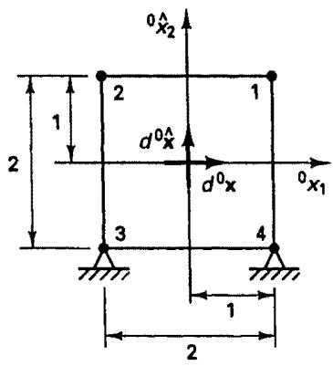# 6.2.4 Exercises 6.1. A four-node plane strain finite element undergoes the deformation shown. The element is originally square, the density $^{0}\rho$ of the element is 0.05, and $d^{0}x$ and $d^{0}\hat{x}$ are infinitesimal fibers. For the deformed configuration at time t: (a) Calculate the displacements of the material points within the element as functions of $^0 x_1$ and $^0 x_2$ . (b) Calculate the deformation gradient ${}^{\prime}X$ , the right Cauchy-Green deformation tensor ${}^{\prime}C$ , and the mass density ${}^{\prime}\rho$ as a function of ${}^{0}x_{1}$ and ${}^{0}x_{2}$ . 

text_image

0^0x^2 1 2 d^0x^0 d^0x 0^0x_1 3 4 1 2


text_image

t_{x2} 2 2 3 30° d_{t,x}^t d_{t,x}^t 1 t_{x1} 4 1 2

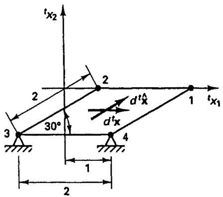
6.2. For the element in Exercise 6.1, calculate the stretches 'λ and 'λ of the line segments $d^{0}x$ and $d^{0}\hat{x}$ and the angular distortion between these line segments. 6.3. Consider the four-node plane strain element shown. Calculate the deformation gradient for times $\Delta t$ and $2\Delta t$ . [Hint: Establish (by inspection) the matrices $\delta\mathbf{R}$ and $\delta\mathbf{U}$ such that $\delta\mathbf{X} = \delta\mathbf{R}$ $\delta\mathbf{U}$ , where $\delta\mathbf{R}$ is an orthogonal (rotation) matrix and $\delta\mathbf{U}$ is a symmetric (stretch) matrix.] 

text_image

Time 0 x2 x1 2 3 45° 2 3 Time Δt 4 Time 2Δt 1.5 45°

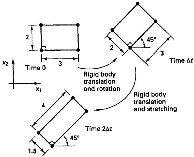
6.4. The four-node plane stress element of incompressible material shown is first stretched in the $x_{1}$ and $x_{2}$ directions and then rigidly rotated by 30 degrees. (a) Calculate the deformation gradient ${}^{2\Delta_{r}}_{0}X$ of the material points in the element. (b) Calculate the stretches of the line elements $d^{0}s_{1}$ and $d^{0}s_{2}$ . 

text_image

x2 2 1 2 d0s2 1 45° d0s1 2 3 4 Time 0 x1 2.5 3 2 1 Time Δt 3 4 2 1 2 4 3 30° Time 2Δt

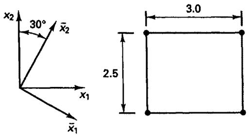
6.5. Consider the four-node element and its deformations to time $\Delta t$ in Exercise 6.4. Assume that the deformation gradient at time $\Delta t$ is now expressed in the coordinate axes $\overline{x}_1$ , $\overline{x}_2$ shown. Calculate this deformation gradient $\Delta t_{0}\overline{\mathbf{X}}$ and show that $\Delta t_{0}\overline{\mathbf{X}}$ is not equal to $^{2\Delta t}_{0}\mathbf{X}$ calculated in Exercise 6.4. (In Exercise 6.4 the element was stretched and rotated, whereas here the element is only stretched.) 

text_image

x₂ 30° x̄₂ x₁ x̄₁ 3.0 2.5

6.6. Consider the motions of two infinitesimal fibers in a two-dimensional continuum. At time 0, the fibers are $$ d ^ {0} \mathbf {x} = \frac {1}{\sqrt {2}} \left[ \begin{array}{l} 1 \\ 1 \end{array} \right] d ^ {0} s; \quad d ^ {0} \hat {\mathbf {x}} = \left[ \begin{array}{l} 0 \\ 1 \end{array} \right] d ^ {0} \hat {s} $$ and at time t, the fibers are $$ d ^ {\prime} \mathbf {x} = \left[ \begin{array}{c} 2 \\ 1 \end{array} \right] d ^ {0} s; \quad d ^ {\prime} \hat {\mathbf {x}} = \left[ \begin{array}{c} - 1 \\ 1 \end{array} \right] d ^ {0} \hat {s} $$ Both fibers emanate from the same material point. (a) Calculate the deformation gradient $\mathbf{0}^{\prime}\mathbf{X}$ at that material point. (b) Calculate the inverse deformation gradient ${}^{0}_{i}X$ at that material point (i) by inverting ${}^{0}_{i}X$ and (ii) without inverting ${}^{0}_{i}X$ . (c) Calculate the mass density ratio $\rho/^{0}\rho$ at the material point. 6.7. Prove that a deformation gradient $\mathbf{X}$ can always be decomposed into the form $\mathbf{X} = \mathbf{V}\mathbf{R}$ where $\mathbf{V}$ is a symmetric matrix and $\mathbf{R}$ is an orthogonal matrix. Establish $\mathbf{V}$ and $\mathbf{R}$ for the deformation in Exercise 6.4. 6.8. A four-node plane strain element is subjected to the following deformations: from time 0 to time $\Delta t$ : $$ \Delta_ {0} \mathbf {U} = \left[ \begin{array}{l l} 2 & 0. 5 \\ 0. 5 & 0. 5 \end{array} \right] $$ from time $\Delta t$ to time $2\Delta t$ : $$ { } ^ { 2 \Delta _ { r } ^ { \prime } } \mathbf { R } = \left[ \begin{array} { c c } \cos 3 0 ^ { \circ } & - \sin 3 0 ^ { \circ } \\ \sin 3 0 ^ { \circ } & \cos 3 0 ^ { \circ } \end{array} \right] $$ (a) Sketch the element and its motions and establish the deformation gradient $^{2\Delta t}_{0}X$ . (b) Calculate the spectral decomposition of $\Delta t\mathbf{U}$ as per (6.32). (c) Calculate the elements of the decomposition of $\mathbf{X} = \mathbf{V}\mathbf{R}$ and interpret this decomposition conceptually. 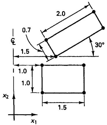6.9. Consider the four-node axisymmetric element shown. Evaluate the deformation gradient and the right and left stretch tensors U, V. 

text_image

2.0 0.7 30° 1.5 1.0 1.0 x2 1.5 x1

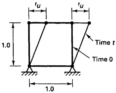
6.10. Consider the motion of the four-node finite element shown. Calculate for time t, (a) The deformation gradient and the polar decompositions $\mathbf{X} = \mathbf{R}\mathbf{U}$ and $\mathbf{X} = \mathbf{V}\mathbf{R}$ (b) The spectral decompositions of $\mathbf{U}$ and $\mathbf{V}$ in (6.32) and (6.33) (c) The velocity strain and spin tensors in (6.42) and (6.43). 

text_image

t_u 1.0 t_u Time t Time 0 1.0

$$ ^ {t} u = 0. 4 $$ $$ ^ {t} \dot {u} = 0. 1; \text { constant velocity } $$ 6.11. Prove the relations in (6.48) to (6.50). 6.12. Prove the relations in (6.56) to (6.61). 6.13. Consider the motion of the four-node element in Exercise 6.10. Calculate $[\dot{\Lambda}]_{\alpha \alpha}$ , $[\Omega_L]_{\alpha \beta}$ , and $[\Omega_E]_{\alpha \beta}$ using the relations (6.48) to (6.50). Verify that (6.46) and (6.47) hold. 6.14. Calculate the components of the Green-Lagrange strain tensors of the elements and their deformations in Exercises 6.1, 6.3, and 6.4. In each case establish the relations in (6.51) and (6.53) to (6.55). 6.15. Calculate the components of the Hencky strain tensor (6.52) for the elements and their deformations in Exercises 6.1, 6.3, and 6.4. 6.16. Consider the element and its motion in Exercise 6.10. For the Green-Lagrange strain and Hencky strain tensors, calculate $E_{g}$ in (6.57) by direct differentiation of (6.56). Also, establish $E_{g}$ using the detailed relations (6.59) to (6.61). 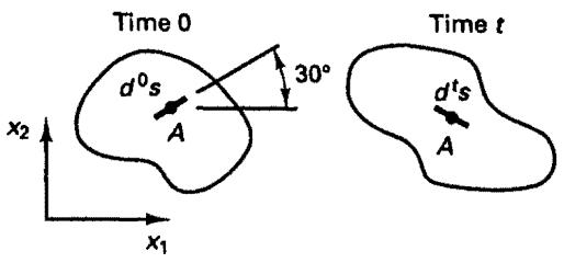6.17. Consider the motion of a material fiber $d^{0}x$ in a body. (a) Prove that for the material fiber the following relation holds using the Green-Lagrange strain tensor $$ _ 0 \epsilon_ {i j} d ^ {0} x _ {i} d ^ {0} x _ {j} = \frac {1}{2} [ (d ^ {t} s) ^ {2} - (d ^ {0} s) ^ {2} ] $$ where $(d^t s)^2 = d^t x_i$ $d^t x_i$ , $(d^0 s)^2 = d^0 x_i$ $d^0 x_i$ and (6.22) is applicable. (b) At point A in a deformed body the Green-Lagrange strain tensor is known to be $$ \mathfrak {d} _ {\epsilon} = \left[ \begin{array}{c c} 0. 6 & 0. 2 \\ 0. 2 & - 0. 3 \end{array} \right] $$ Find the stretch $t\lambda$ of the line element $d^0 s = \| d^0\mathbf{x} \|_2$ shown. Can you calculate the rotation of the line element? Explain your answer. 

text_image

Time 0 30° d⁰s A x₂ x₁ Time t dᵗs A

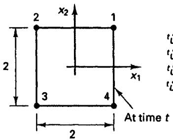
6.18. The nodal point velocities of a four-node element are as shown. Using the element interpolation functions, evaluate the components of the velocity strain tensor and spin tensor of the element. Physically explain why your answer is correct. 

text_image

2 x₂ 1 2 x₁ 3 4 2 At time t

$$ \begin{array}{l} { } ^ { t } \dot { u } _ { 1 } ^ { 1 } = 0 . 2 ; \quad { } ^ { t } \dot { u } _ { 2 } ^ { 1 } = 0 . 1 \\ { } ^ { t } \dot { u } _ { 1 } ^ { 2 } = - 0 . 1 ; \quad { } ^ { t } \dot { u } _ { 2 } ^ { 2 } = - 0 . 2 \\ { } ^ { t } \dot { u } _ { 1 } ^ { 3 } = - 0 . 2 ; \quad { } ^ { t } \dot { u } _ { 2 } ^ { 3 } = - 0 . 1 \\ { } ^ { t } \dot { u } _ { 1 } ^ { 4 } = 0 . 1 ; \quad { } ^ { t } \dot { u } _ { 2 } ^ { 4 } = 0 . 2 \\ \end{array} $$ 6.19. Consider the four-node plane strain element and its motion in Exercise 6.10. Evaluate the components $^{t}D_{mn}$ using the relation (6.64). 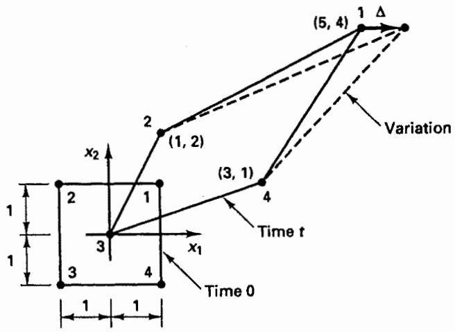6.20. Consider the four-node plane strain element shown. Evaluate the components of the tensor $\delta_{t}e_{mn}$ corresponding to the virtual displacement $\delta u_{1}^{k} = \Delta$ at node 1 as a function of $^0 x_1$ and $^0 x_2$ . (All other $\delta u_{j}^{k} = 0$ .) Evaluate all matrix expressions required but do not necessarily perform the matrix multiplications. 

text_image

x2 1 2 (1, 2) 2 (5, 4) 1 Δ Variation (3, 1) 4 Time t x1 3 4 Time 0 1 1

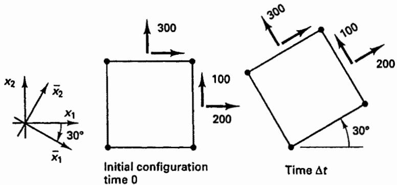
6.21. Consider the four-node element shown, subjected to an initial stress with components $$ \begin{array}{l} \text { Initial stress } \\ \text {(stress at time 0)} \end{array} = \mathbf {0} \mathbf {S} \equiv \mathbf {0} _ {\mathbf {T}} = \left[ \begin{array}{l l} 2 0 0 & 1 0 0 \\ 1 0 0 & 3 0 0 \end{array} \right] $$ The element is undeformed in its initial configuration. Assume that the element is subjected to a counterclockwise rigid body rotation of 30 degrees from time 0 to time $\Delta t$ . (a) Calculate the Cauchy stresses $\Delta\tau$ corresponding to the stationary coordinate system $x_{1}, x_{2}$ . (b) Calculate the second Piola-Kirchhoff stresses $\Delta_{0}^{\prime}\mathbf{S}$ corresponding to $x_{1}, x_{2}$ . (c) Calculate the deformation gradient $\Delta t_{0}X$ . 

text_image

x2 x̅2 x1 30° x̅1 300 100 200 Initial configuration time 0 300 100 200 30° Time Δt

Next, assume that the element remains in its initial configuration but the coordinate system is rotated clockwise by 30 degrees. (d) Calculate the Cauchy stresses ${}^{0}\overline{\tau}$ corresponding to $\overline{x}_{1}, \overline{x}_{2}$ . (e) Calculate the second Piola-Kirchhoff stresses $\mathbb{S}$ corresponding to $\overline{x}_1, \overline{x}_2$ . (f) Calculate the deformation gradient $\mathfrak{g}\overline{\mathbf{X}}$ corresponding to $\overline{x}_1, \overline{x}_2$ .