# Chapter 5 # Elasto-plastic Timoshenko beam analysis Written in collaboration with H. H. Abdel Rahman # 5.1 Introduction In this chapter we introduce some elastoplastic beam formulations which are useful in their own right but which also provide insight into the elastoplastic plate formulations presented later. There are two main beam theories on which we could base our studies: (i) Euler–Bernoulli beam theory. This theory, which is usually favoured by engineers because of its simplicity, takes no account of transverse shear deformation. The simplest Euler–Bernoulli beam element based on the displacement method is the well-known Hermitian element $^{(1)}$ with cubic displacements. Bending moments may vary linearly over this element. (ii) Timoshenko beam theory. This theory allows for transverse shear deformation effects. The simplest Timoshenko beam element is the Hughes element $^{(2)}$ with linear displacements and normal rotations. Bending moments are constant over this element. Although the Euler–Bernoulli theory is frequently adopted we choose the Timoshenko beam theory as a basis for our study of the elasto-plastic analysis of beams since we may make use of a finite element which involves constant bending moments and is more in keeping with the presentations given in the previous chapters. Furthermore, Timoshenko beam theory can rightly be considered as the one-dimensional precursor of Mindlin plate theory which is used in Chapter 9. Firstly in this chapter the basic assumptions of Timoshenko beam theory are outlined. The Hughes element formulation is then presented for the elastic case. There are two approaches to the elasto-plastic analysis of Timoshenko beams: (i) Non-layered approach. In this method, when the bending moment reaches the yield moment, the whole cross-section of the beam is assumed to become plastic instantaneously. This is however a convenient fiction as in reality there is always a gradual plastification of the beam with the outer fibres becoming plastic initially. The zone of plasticification then spreads inwards until the whole section ultimately becomes plastic. (ii) Layered approach. In this method we attempt to capture the spread of plasticity over the depth of the beam. The beam is thus divided into a number of layers each of which may become plastic separately. As the number of layers is increased, this model provides a more realistic representation of the gradual spread of plasticity over the beam cross-section. Both non-layered and layered approaches are described in detail and program TIMOSH for the non-layered beams and program TIMLAY for the layered beams are presented and their use is illustrated with the aid of some examples. # 5.2 The basic assumptions of Timoshenko beam theory # 5.2.1 Introductory comments There are several basic assumptions adopted-in the derivation of the governing equations of Timoshenko beam theory. Here we reiterate these assumptions for elastic, small deflection analysis and then in later sections we present some extensions of the theory to allow for elasto-plastic analysis. 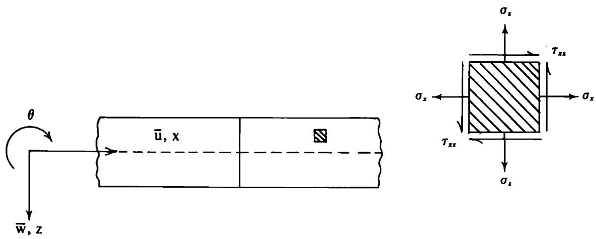# 5.2.2 Assumed displacement field In a typical Timoshenko beam, such as the one shown in Fig. 5.1, it is usual to assume that normals to the neutral axis before deformation remain straight but not necessarily normal to the neutral axis after deformation. This implies that the axial displacement $\bar{u}$ at any point $(x, z)$ may be expressed directly in terms of $\theta(x)$ the rotation of the normal so that $$ \bar {u} (x, z) = - z \theta (x) \tag {5.1} $$ Note that the normal rotation $\theta(x)$ is equal to the slope of the neutral axis dw/dx minus a rotation $\beta$ which is due to the transverse shear deformation. 

text_image

θ ū, x w, z σₓ τₓₓ σₓ τₓₓ σₓ σₓ

Fig. 5.1 Timoshenko beam. Thus we have $$ \theta (x) = \frac {d \bar {w}}{d x} - \beta . \tag {5.2} $$ Notice also that the lateral displacement $\bar{w}$ at any point $(x, z)$ is given by the lateral displacement at the neutral axis so that $$ \bar {w} (x, z) = w (x) \tag {5.3} $$ # 5.2.3 Stress-strain relationships In Timoshenko beam theory, the elastic stress–strain relationships used for plane stress analysis are usually adopted in a slightly modified form. For convenience we assume that the beam is loaded in the xz plane and thus for an isotropic elastic material the relevant stress–strain relationships are $$ \left[ \begin{array}{l} \sigma_ {x} \\ \sigma_ {z} \\ \tau_ {x z} \end{array} \right] = \frac {E}{(1 - \nu^ {2})} \left[ \begin{array}{c c c} 1 & \nu & 0 \\ \nu & 1 & 0 \\ 0 & 0 & \frac {(1 - \nu)}{2} \end{array} \right] \left[ \begin{array}{l} \epsilon_ {x} \\ \epsilon_ {z} \\ \gamma_ {x z} \end{array} \right] \tag {5.4} $$ where $E$ is the Young's modulus and $\nu$ is the Poisson's ratio. If $\sigma_z$ is assumed to be equal to zero then $$ \epsilon_ {z} = - \nu \epsilon_ {x} \tag {5.5} $$ and by eliminating $\epsilon_{z}$ from (5.4) and (5.5), it is possible to write the following stress-strain relationship $$ \sigma_ {x} = E \epsilon_ {x} \quad \text { and } \quad \tau_ {x z} = G \gamma_ {x z} \tag {5.6} $$ where for an isotropic material $G = E / [2(1 + \nu)]$ is the shear modulus. # 5.2.4 Strain-displacement relationships Usually small deflection theory is adopted and the axial strain $\epsilon_{x}$ is given as $$ \epsilon_ {x} = \frac {\dot {c} \bar {u}}{\dot {c} x}. \tag {5.7} $$ If approximation (5.1) is adopted then this strain can be written as $$ \epsilon_ {x} = - z \frac {d \theta}{d x}. \tag {5.8} $$ Similarly the shear strain $\gamma_{xz}$ is given as $$ \gamma_ {x z} = \frac {\dot {c} \bar {u}}{\dot {c} z} + \frac {\dot {c} \bar {w}}{\dot {c} x} \tag {5.9} $$ and if approximation (5.2) is adopted we obtain $$ \gamma_ {x z} = - \theta + \frac {d w}{d x} = \beta . \tag {5.10} $$ # 5.2.5 Virtual work expression Consider a Timoshenko beam of depth t in which the breadth b varies with depth symmetrically about the neutral axis. The beam is subjected to a distributed loading of intensity q. If the beam undergoes a set of virtual lateral displacements $\delta w$ , virtual normal rotations $\delta\theta$ and associated virtual curvatures $-z[d(\delta\theta)/dx]$ and virtual shear strains $\delta\beta$ then the virtual work equation can be written as $$ \int_ {0} ^ {l} \int_ {- t / 2} ^ {t / 2} \int_ {b (- t / 2)} ^ {b (t / 2)} \left\{- z \frac {d (\delta \theta)}{d x} \sigma_ {x} + \delta \beta \tau_ {x z} \right\} d y d z d x - \int_ {0} ^ {l} \delta w q d x = 0 \tag {5.11} $$ or $$ \int_ {0} ^ {l} \left(- \frac {d (\delta \theta)}{d x} M + \delta \beta Q\right) d x - \int_ {0} ^ {l} \delta w q d x = 0 $$ where the bending moment $$ M = \int_ {- t / 2} ^ {t / 2} \int_ {b (- t / 2)} ^ {b (t / 2)} z \sigma_ {x} d y d z \tag {5.12} $$ and the shear force $$ Q = \int_ {- t / 2} ^ {t / 2} \int_ {b (- t / 2)} ^ {b (t / 2)} \tau_ {x z} d y d z. \tag {5.13} $$ Using (5.12) and (5.13), if we substitute for $\sigma_x$ and $\tau_{xz}$ in (5.6) respectively we obtain $$ M = \left(\int_ {- t / 2} ^ {t / 2} \int_ {b (- t / 2)} ^ {b (t / 2)} z ^ {2} E d y d z\right) \left(- \frac {d \theta}{d x}\right) = E I \left(- \frac {d \theta}{d x}\right) \tag {5.14} $$ and $$ Q = \left(\int_ {- t / 2} ^ {t / 2} \int_ {b (- t / 2)} ^ {b (t / 2)} G d y d z\right) (\beta) = G A \beta \tag {5.15} $$ where $EI$ is the flexural rigidity and $GA$ , the shear rigidity, is replaced by $GA$ where the area $A$ is replaced by $A/\alpha$ . The parameter $\alpha$ is a correction factor to allow for cross-sectional warping. For a rectangular section $\alpha$ is usually taken as 1·5.\* \* Many different definitions of $\alpha$ have been presented in the various papers on Timoshenko beams. Cowper $^{(3)}$ summarises some definitions for beams of various cross-sections. For example, he shows that $\alpha$ may be taken as $(12 + 11\nu)/(10 + 10\nu)$ for rectangular cross-sections and $(7 + 6\nu)/(6 + 6\nu)$ for circular cross-sections. Here we take $\alpha = 1 \cdot 5$ unless otherwise stated. If we substitute for $M$ and $Q$ from (5.14) and (5.15) we can rewrite the virtual work equation (5.11) as $$ \int_ {0} ^ {l} \left(\frac {d (\delta \theta)}{d x} E I \frac {d \theta}{d x} + \delta \beta G \hat {A} \beta - \delta w q\right) d x = 0 \tag {5.16} $$ # 5.2.6 A comparison of various beam approximations In order to compare the various beam approximations consider a simply supported beam of rectangular cross-section, flexural rigidity $EI$ , Poisson's ratio $\nu$ , depth $t$ and length $L$ which is subjected to a uniformly distributed loading $q$ . The lateral deflection in the elastic range is given as $$ w = \frac {q L ^ {4}}{2 4 E I} \left\{\left[ \left(\frac {x}{L}\right) ^ {4} - \frac {3}{2} \left(\frac {x}{L}\right) ^ {2} + \frac {5}{1 6} \right] + \left(\frac {t}{L}\right) ^ {2} \left[ \frac {1 2}{5} + \frac {3 \nu}{2} \right] \left[ \frac {1}{4} - \left(\frac {x}{L}\right) ^ {2} \right] \right\} \tag {5.17a} $$ when plane stress (PS) assumptions are adopted, $$ w = \frac {q L ^ {4}}{2 4 E I} \left\{\left[ \left(\frac {x}{L}\right) ^ {4} - \frac {3}{2} \left(\frac {x}{L}\right) ^ {2} + \frac {5}{1 6} \right] + \left(\frac {t}{L}\right) ^ {2} [ 2 a (1 + \nu) ] \left[ \frac {1}{4} - \left(\frac {x}{L}\right) ^ {2} \right] \right\} \tag {5.17b} $$ when Timoshenko beam (TB) assumptions are adopted and $$ w = \frac {q L ^ {4}}{2 4 E I} \left\{\left[ \left(\frac {x}{L}\right) ^ {4} - \frac {3}{2} \left(\frac {x}{L}\right) ^ {2} + \frac {5}{1 6} \right] \right\} \tag {5.17c} $$ when Euler–Bernoulli (EB) assumptions are adopted. Thus, for long slender beams in which $(t/L)$ is small, EB theory is adequate. If we take Cowper's value ${}^{(3)}$ of $\alpha = (12 + 11\nu)/(10 + 10\nu)$ then the ratio of the second-order additional lateral deflections due to shear deformation obtained under TB and PS assumptions is $(24 + 22\nu)/(24 + 15\nu)$ which varies from 1·00 to 1·11 as $\nu$ varies from 0·0 to 0·5. Thus TB theory is an accurate theory for beams of all dimensions. # 5.3 Finite element idealisation for linear elastic Timoshenko beams # 5.3.1 Introduction The theoretical and programming aspects of the finite element analysis of linear elastic Timoshenko beams have been dealt with in detail in previous books by the authors $^{(1, 5)}$ . Here we derive the stiffness matrix and consistent load vector for a linear element and set the scene for the analysis of elasto-plastic Timoshenko beams which will be discussed later. 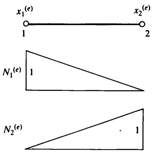# 5.3.2 Displacement and strain representation In the Hughes element representation, the lateral displacement w is represented by the relationship $$ w ^ {(e)} = N _ {1} ^ {(e)} w _ {1} ^ {(e)} + N _ {2} ^ {(e)} w _ {2} ^ {(e)} \tag {5.18} $$ where $w_{1}^{(e)}$ and $w_{2}^{(e)}$ are the nodal lateral displacements at local nodes 1 and 2 of element e and the shape functions (shown in Fig. 5.2) are $$ N _ {1} ^ {(e)} = \left(x _ {2} ^ {(e)} - x ^ {(e)}\right) / l ^ {(e)} $$ and $$ N _ {2} ^ {(e)} = \left(x ^ {(e)} - x _ {1} ^ {(e)}\right) / l ^ {(e)} $$ in which $x_{1}^{(e)}$ and $x_{2}^{(e)}$ are the x-coordinates of local nodes 1 and 2, $x^{(e)}$ is the x-coordinate of a point within the element and $l^{(e)}$ is the length of the element. 

text_image

x₁⁽ᵉ⁾ 1 x₂⁽ᵉ⁾ 2 N₁⁽ᵉ⁾ 1 N₂⁽ᵉ⁾ 1

Fig. 5.2 Beam element shape functions. Similarly the normal rotation $\theta^{(e)}$ within element e is represented as $$ \theta^ {(e)} = N _ {1} ^ {(e)} \theta_ {1} ^ {(e)} + N _ {2} ^ {(e)} \theta_ {2} ^ {(e)} \tag {5.19} $$ where $\theta_{1}^{(e)}$ and $\theta_{2}^{(e)}$ are the normal rotations at local nodes 1 and 2 of element $e$ . The curvature-displacement relationship can be expressed as $$ - \left(\frac {d \theta}{d x}\right) ^ {(e)} = - \left(\frac {d N _ {1}}{d x}\right) ^ {(e)} \theta_ {1} ^ {(e)} - \left(\frac {d N _ {2}}{d x}\right) ^ {(e)} \theta_ {2} ^ {(e)} \tag {5.20} $$ or $$ \epsilon_ {f} ^ {(e)} = \left[ 0, \frac {1}{l ^ {(e)}}, 0, - \frac {1}{l ^ {(e)}} \right] \left[ \begin{array}{l} w _ {1} ^ {(e)} \\ \theta_ {1} ^ {(e)} \\ w _ {2} ^ {(e)} \\ \theta_ {2} ^ {(e)} \end{array} \right] = \boldsymbol {B} _ {f} ^ {(e)} \boldsymbol {\varphi} ^ {(e)} $$ where $B_{f}^{(e)}$ is the curvature–displacement matrix. The shear strain-displacement relationship is given as $$ \left(\frac {d w}{d x} - \theta\right) ^ {(e)} = \left(\frac {d N _ {1}}{d x}\right) ^ {(e)} w _ {1} ^ {(e)} - N _ {1} ^ {(e)} \theta_ {1} ^ {(e)} + \left(\frac {d N _ {2}}{d x}\right) ^ {(e)} w _ {2} ^ {(e)} - N _ {2} ^ {(e)} \theta_ {2} ^ {(e)} \tag {5.21} $$ or $$ \epsilon_ {s} ^ {(e)} = \left[ - \frac {1}{l ^ {(e)}}, - \frac {\left(x _ {2} ^ {(e)} - x ^ {(e)}\right)}{l ^ {(e)}}, \frac {1}{l ^ {(e)}}, - \frac {\left(x ^ {(e)} - x _ {1} ^ {(e)}\right)}{l ^ {(e)}} \right] \left[ \begin{array}{l} w _ {1} ^ {(e)} \\ \theta_ {1} ^ {(e)} \\ w _ {2} ^ {(e)} \\ \theta_ {2} ^ {(e)} \end{array} \right] = \boldsymbol {B} _ {s} ^ {(e)} \boldsymbol {\varphi} ^ {(e)} $$ where $B_{s}^{(e)}$ is the shear strain–displacement matrix. # 5.3.3 Stiffness matrix evaluation Given the element strain-displacement relationships outlined in Section 5.3.2, Hughes has shown that using a virtual work approach the governing equations can be expressed as $$ [ \boldsymbol {K} _ {f} + \boldsymbol {K} _ {s} ] \varphi - \boldsymbol {f} = 0 \tag {5.22} $$ where the submatrices of $K_{f}$ and $K_{s}$ and subvectors of f for element e can be written as $$ \boldsymbol {K} _ {f} ^ {(e)} = \int_ {X _ {1} ^ {(e)}} ^ {X _ {2} ^ {(e)}} [ \boldsymbol {B} _ {f} ^ {(e)} ] ^ {T} (E I) ^ {(e)} \boldsymbol {B} _ {f} ^ {(e)} d x $$ $$ \boldsymbol {K} _ {s} ^ {(e)} = \int_ {X _ {1} ^ {(e)}} ^ {X _ {2} ^ {(e)}} [ \boldsymbol {B} _ {s} ^ {(e)} ] ^ {T} (G \hat {A}) ^ {(e)} \boldsymbol {B} _ {s} ^ {(e)} d x $$ $$ \boldsymbol {f} ^ {(e)} = \int_ {X _ {1} ^ {(e)}} ^ {X _ {2} ^ {(e)}} [ N _ {1} ^ {(e)}, 0, N _ {2} ^ {(e)}, 0 ] ^ {T} q d x. \tag {5.23} $$ The flexural element stiffness matrix can be evaluated using a 1-point Gauss–Legendre rule and takes the form $$ \boldsymbol {K} _ {f} ^ {(e)} = \left(\frac {E I}{l}\right) ^ {(e)} \left[ \begin{array}{c c c c} 0 & 0 & 0 & 0 \\ 0 & 1 & 0 & - 1 \\ 0 & 0 & 0 & 0 \\ 0 & - 1 & 0 & 1 \end{array} \right] \tag {5.24} $$ If $K_{s}^{(e)}$ is evaluated exactly using a 2-point Gauss–Legendre rule we obtain $$ \boldsymbol {K} _ {s} ^ {(e)} = \left(\frac {G \hat {A}}{l}\right) ^ {(e)} \left[ \begin{array}{c c c c} 1 & \frac {l}{2} & - 1 & \frac {l}{2} \\ \frac {l}{2} & \frac {l ^ {2}}{3} & - \frac {l}{2} & \frac {l ^ {2}}{6} \\ - 1 & - \frac {l}{2} & 1 & - \frac {l}{2} \\ \frac {l}{2} & \frac {l ^ {2}}{6} & - \frac {l}{2} & \frac {l ^ {2}}{3} \end{array} \right] ^ {(e)} \tag {5.25} $$ Unfortunately it has been shown that with this formulation, overstiff solutions are obtained. This phenomenon, known as locking, may be 'cured' by integrating $K_{s}^{(e)}$ with a 1-point Gauss-Legendre rule. If such a selectively integrated element is adopted we find that $$ \boldsymbol {K} _ {s} ^ {(e)} = \left(\frac {G \hat {A}}{l}\right) ^ {(e)} \left[ \begin{array}{c c c c} 1 & \frac {l}{2} & - 1 & \frac {l}{2} \\ \frac {l}{2} & \frac {l ^ {2}}{4} & - \frac {l}{2} & \frac {l ^ {2}}{4} \\ - 1 & - \frac {l}{2} & 1 & - \frac {l}{2} \\ \frac {l}{2} & \frac {l ^ {2}}{4} & - \frac {l}{2} & \frac {l ^ {2}}{4} \end{array} \right] ^ {(e)} \tag {5.26} $$ and the results obtained are excellent. The consistent nodal force vector is given as $$ f ^ {(e)} = \left[ \frac {(q l) ^ {(e)}}{2}, 0, \frac {(q l) ^ {(e)}}{2}, 0 \right] \tag {5.27} $$ which, unlike the Euler–Bernōulli cubic Hermitian element, only has lateral nodal point forces. For the nonlayered elasto-plastic Timoshenko beam finite element analysis, when the beam bending moment reaches the yield moment $M_{0}$ , the whole element becomes plastic and acts as a plastic hinge. In such a situation the flexural rigidity EI is replaced by an elasto-plastic flexural rigidity $(EI)_{ep}$ whereas the shear rigidity $G\hat{A}$ is assumed to be unchanged. # 5.3.4 Element stress resultants We can obtain expressions which enable us to calculate the bending moments and shear forces within each element using $(5.14)$ and $(5.15)$ . The bending moment, which is constant in each element $e$ , is given as $$ \begin{array}{l} M ^ {(e)} = (E I) ^ {(e)} B _ {f} ^ {(e)} \varphi^ {(e)} = (E I) ^ {(e)} \left[ 0, \frac {1}{l ^ {(e)}}, 0, - \frac {1}{l ^ {(e)}} \right] \left[ \begin{array}{l} w _ {1} ^ {(e)} \\ \theta_ {1} ^ {(e)} \\ w _ {2} ^ {(e)} \\ \theta_ {2} ^ {(e)} \end{array} \right] \\ = \left(\frac {E I}{l}\right) ^ {(e)} \left(\theta_ {1} ^ {(e)} - \theta_ {2} ^ {(e)}\right). \tag {5.28} \\ \end{array} $$ The shear force varies linearly over each element but we evaluate it at $$ x = \frac {x _ {1} ^ {(e)} + x _ {2} ^ {(e)}}{2} $$ and assume it to be constant over the element. This is consistent with the practice of using selective integration in the evaluation of $K^{(e)}$ . The shear force is therefore given as $$ \begin{array}{l} \begin{array}{l} Q ^ {(e)} = (G \hat {A}) ^ {(e)} B _ {s} ^ {(e)} \varphi^ {(e)} = (G \hat {A}) ^ {(e)} \left[ - \frac {1}{l ^ {(e)}}, - \frac {1}{2}, \frac {1}{l ^ {(e)}}, - \frac {1}{2} \right] \left[ \begin{array}{l} w _ {1} ^ {(e)} \\ \theta_ {1} ^ {(e)} \\ w _ {2} ^ {(e)} \\ \theta_ {2} ^ {(e)} \end{array} \right] \\ \left(\left. w _ {2} ^ {(e)} - w _ {1} ^ {(e)}\right) \left. \left. \left. \left. \theta_ {1} ^ {(e)} + \theta_ {2} ^ {(e)}\right) \right. \right. \right. \right. \end{array} \\ = (G \hat {A}) ^ {(e)} \left\{\left(\frac {w _ {2} ^ {(e)} - w _ {1} ^ {(e)}}{l ^ {(e)}}\right) - \left(\frac {\theta_ {1} ^ {(e)} + \theta_ {2} ^ {(e)}}{2}\right) \right\}. \tag {5.29} \\ \end{array} $$ # 5.4 Elasto-plastic nonlayered Timoshenko beams # 5.4.1 The yield moment Consider a Timoshenko beam subjected to a bending moment. Timoshenko's assumptions imply that the axial stress and strain vary linearly across the depth of the section. As the bending moment is increased the yield stress is attained at the top and bottom fibres and with a further increase the yield will spread from these outer fibres inwards until the two zones of yield meet. The cross-section is then said to be fully plastic. It should be noted that the interaction of $\sigma_{x}$ and $\tau_{xz}$ has been ignored during yield. This is inexact, but experience shows that the effect is not of prime importance especially when thin beams are considered. The value of this ultimate moment in the fully plastic condition can be calculated in terms of the yield stress $\sigma_{0}$ .\* Thus $$ M _ {0} = \int_ {b (- t / 2)} ^ {b (t / 2)} \int_ {- t / 2} ^ {t / 2} z \sigma_ {0} d z d y \tag {5.30} $$ \* Note that for beam and plate problems the uniaxial yield stress is designated by $\sigma_0$ and not $\sigma_Y$ . and for a rectangular beam of breadth b, $M_{0} = \sigma_{0}(bt^{2}/4)$ . However, it should be noted that the assumption used in the finite element solution implies that the whole cross-section becomes plastic as soon as the bending moment reaches its yield value $M_{0}$ . This means that, for the beam case shown in Fig. 5.3, the whole cross-section is assumed to be plastic when the bending moment of situation (c) becomes equal to the bending moment of situation (d)—in which case the extreme fibre stress in situation (c) exceeds the actual yield stress of the material.  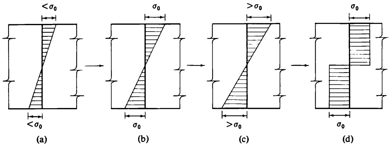Fig. 5.3 Yielding of non-layered beam. # 5.4.2 Elasto-plastic bending As mentioned earlier, elasto-plastic behaviour is characterised by an initial elastic material response with an additional plastic deformation when the bending moment $|M|$ exceeds the yield moment $M_{0}$ . The plastic deformation is irreversible on unloading and its onset is governed by a very simple yield criterion. Post-yield deformation usually occurs with a considerably reduced material stiffness. The moment-curvature relationship for a Timoshenko beam of elastoplastic material is shown in Fig. 5.4. The beam initially deforms elastically with a flexural rigidity of EI until the ultimate bending moment is reached at which stage the whole beam cross-section becomes plastic. On increasing the load further, the material is assumed to exhibit linear strain-hardening characterised by the tangential flexural rigidity $(EI)_{T}$ . At some stage after initial yielding consider a further load application resulting in an incremental increase of bending moment accompanied by a change of curvature $d\epsilon_{f}$ . Assuming that the curvature can be separated into elastic and plastic components, so that $$ d \epsilon_ {f} = (d \epsilon_ {f}) _ {e} + (d \epsilon_ {f}) _ {p}, \tag {5.31} $$ we define as a strain hardening parameter