![](images/page-141_c042553ebb990b23668258faec308a872c2aa80b6406581530e4a7a60cf59d2e.jpg)
line | Curvature | Bending Moment | Slope EI | | --------- | -------------- | -------- | | dεf | 0 | 0 | | dεf | M0 | (dεf)e | | dεf | (dεf)p | (dεf)p |
Fig. 5.4 Moment curvature relationship for a Timoshenko beam. $$ H ^ {\prime} = \frac {d M}{(d \epsilon_ {f}) _ {p}}. $$ This can be interpreted as the slope of the strain-hardening portion of the moment-curvature curve after the removal of the elastic curvature component. Thus $$ H ^ {\prime} = \frac {d M}{d \epsilon_ {f} - (d \epsilon_ {f}) _ {e}} = \frac {(E I) _ {T}}{1 - [ (E I) _ {T} / E I ]}. \tag {5.32} $$ It is therefore possible to rewrite (5.31) as $$ d \epsilon_ {f} = \frac {d M}{E I} + \frac {d M}{H ^ {\prime}} = \frac {d M (H ^ {\prime} + E I)}{E I H ^ {\prime}} \tag {5.33} $$ and then the incremental moment–curvature relationship can be written in the form $$ d M = \frac {E I H ^ {\prime}}{(E I + H ^ {\prime})} d \epsilon_ {f}. \tag {5.34} $$ Thus during yielding the incremental stress–strain resultant relationship is $$ d M = E I \left(1 - \frac {E I}{E I \pm H ^ {\prime}}\right) d \epsilon_ {f} $$ $$ d Q = G \hat {A} d \epsilon_ {s}. \tag {5.35} $$ The shear force/shear strain relationship is always elastic whereas the moment–curvature relationship is elasto-plastic. After yielding the flexural rigidity EI is replaced by $$ E I \left(1 - \frac {E I}{E I + H ^ {\prime}}\right). $$ If the hardening parameter $H'$ is equal to zero then the material behaviour is elasto-perfectly plastic and as mentioned in Section 3.5 for elasto-plastic axial bar elements this may lead to tangential stiffness matrices which are singular. This difficulty can also be avoided by use of the initial stiffness method in which the elastic element stiffnesses are employed at every stage of the computation thereby guaranteeing a positive definite assembled stiffness matrix. # 5.4.3 Solution of nonlinear equations Let us now generate the nonlinear equilibrium equations using the virtual expression (5.11). In order to do this we require the global rather than the element expressions for the lateral displacements, rotation, curvature and shear strain. At any point in the finite element mesh the lateral displacement and rotation can be obtained from the expression $$ \left[ \begin{array}{l} w \\ \theta \end{array} \right] = N \varphi \tag {5.36} $$ where the shape function matrix is $$ N = \left[ \begin{array}{l l l l l l} N _ {1}, & 0, & N _ {2}, & 0, & \dots , & N _ {n}, & 0 \\ 0, & N _ {1}, & 0, & N _ {2}, & \dots , & 0, & N _ {n} \end{array} \right] \tag {5.37} $$ and the vector of nodal displacements is $$ \varphi = [ w _ {1}, \theta_ {1}, w _ {2}, \theta_ {2}, \dots , w _ {n}, \theta_ {n} ] ^ {T} \tag {5.38} $$ where $w_{i}$ , $\theta_{i}$ and $N_{i}$ are the lateral displacement, rotation and global shape functions associated with node i. The curvature and shear strain at any point within the entire finite element mesh is given as $$ - \frac {d \theta}{d x} = B _ {f} \varphi \quad \text { and } \quad \frac {d w}{d x} - \theta = B _ {s} \varphi \tag {5.39} $$ where $$ \boldsymbol {B} _ {f} = \left[ 0, - \frac {d N _ {1}}{d x}, 0, - \frac {d N _ {2}}{d x}, \dots , 0, - \frac {d N _ {n}}{d x} \right] \tag {5.40} $$ and $$ \boldsymbol {B} _ {s} = \left[ \frac {d N _ {1}}{d x}, - N _ {1}, \frac {d N _ {2}}{d x}, - N _ {2}, \dots , \frac {d N _ {n}}{d x}, - N _ {n} \right] \tag {5.41} $$ Virtual curvatures and shear strains are given as $$ - \frac {d (\delta \theta)}{d x} = \boldsymbol {B} _ {f} \delta \varphi \quad \text { and } \quad \frac {d (\delta w)}{d x} - \delta \theta = \boldsymbol {B} _ {s} \delta \varphi \tag {5.42} $$ respectively, where the vector of virtual nodal displacements is written as $$ \delta \varphi = [ \delta w _ {1}, \delta \theta_ {1}, \delta w _ {2}, \delta \theta_ {2}, \dots , \delta w _ {n}, \delta \theta_ {n} ] ^ {T}. \tag {5.43} $$ Thus the virtual work expression (5.11) can now be written as $$ \begin{array}{l} \int_ {0} ^ {l} [ \delta \varphi ] ^ {T} [ \boldsymbol {B} _ {f} ] ^ {T} M d x + \int_ {0} ^ {l} [ \delta \varphi ] ^ {T} [ \boldsymbol {B} _ {s} ] ^ {T} Q d x \\ - \int_ {0} ^ {l} [ \delta \varphi ] ^ {T} [ \bar {\mathbf {N}} ] ^ {T} q d x = 0 \tag {5.44} \\ \end{array} $$ where $\bar{\mathbf{N}} = [N_1, 0, N_2, 0, \dots, N_n, 0]$ . (5.45) Since (5.44) must be true for any set of virtual displacements $\delta \varphi$ then we have $$ \left\{\int_ {0} ^ {l} \left[ \boldsymbol {B} _ {f} \right] ^ {T} M d x + \int_ {0} ^ {l} \left[ \boldsymbol {B} _ {s} \right] ^ {T} Q d x \right\} - \int_ {0} ^ {l} \left[ \bar {\mathbf {N}} \right] ^ {T} q d x = 0 \tag {5.46} $$ or $$ p - f = 0. $$ In fact this equation is identical to (5.22) when there is no plasticity. Unfortunately in elasto-plastic problems M is a nonlinear function and in general we can only predict the vector p approximately. Thus (5.46) is nonlinear and since p is only approximately known than p-f will equal a residual value $\psi(\varphi)$ which we attempt to reduce to zero in our solution procedure. We evaluate contributions to p element by element and assemble in the usual manner. The contribution from element e has the form $$ \begin{array}{l} \boldsymbol {p} ^ {(e)} = \int_ {x _ {1} ^ {(e)}} ^ {x _ {2} ^ {(e)}} \left[ \begin{array}{c} 0 \\ \frac {1}{l ^ {(e)}} \\ 0 \\ - \frac {1}{l ^ {(e)}} \end{array} \right] M ^ {(e)} d x + \int_ {x _ {1} ^ {(e)}} ^ {x _ {2} ^ {(e)}} \left[ \begin{array}{c} - \frac {1}{l ^ {(e)}} \\ \frac {x ^ {(e)} - x _ {2} ^ {(e)}}{l ^ {(e)}} \\ \frac {1}{l ^ {(e)}} \\ \frac {x _ {1} ^ {(e)} - x ^ {(e)}}{l ^ {(e)}} \end{array} \right] Q ^ {(e)} d x \\ = \left[ - Q ^ {(e)}, M ^ {(e)} - \frac {(Q l) ^ {(e)}}{2}, Q ^ {(e)}, - M ^ {(e)} - \frac {(Q l) ^ {(e)}}{2} \right] ^ {T}. \tag {5.47} \\ \end{array} $$ \*The second integral evaluation is equivalent to using a 1-point Gauss rule. ![](images/page-144_286badf9fdf174f5c6d48de7f661af3aedd8e1501ccaa009f381fe58e33ee0b8.jpg)
flowchart ```mermaid graph TD A["DATA"] --> B["Input data defining geometry, loading and boundary conditions, material properties, etc."] B --> C["INITAL"] C --> D["Input data for current increment."] D --> E["INCREM"] E --> F["Initialize accumulative arrays to zero. Update load vector."] F --> G["NONAL"] G --> H["Set indicator to identify type of solution algorithm."] H --> I{Is new element stiffness matrix required?} I -->|No| J["No"] I -->|Yes| K["STIFFB"] K --> L["Calculate the element stiffness matrices and store on disc."] L --> M["ASSEMB and GREDUC or RESOLV and BAKSUB"] M --> N["Assemble global stiffness matrix (or take previous one) and global load vector and solve the resulting equations for unknowns."] N --> O["REFORB"] O --> P["Calculate the residual force vector."] P --> Q["CONUND"] Q --> R["Has solution converged?"] R -->|No| S["No"] R -->|Yes| T["RESULT"] T --> U["Output the results."] U --> V["END"] V --> W["LOAD INCREMENT LOOP"] W --> X["ITERATION LOOP"] ```
Fig. 5.5 Overall structure of program TIMOSH. Note that the appropriate value of bending moment $M^{(e)}$ is inserted in (5.47). Table 5.1 shows the complete sequence of nonlinear equation solving which is very similar to the one adopted for the axially-loaded bars in Chapter 3. 1. Begin load increment. Set $f = f + \Delta f$ , iteration counter i = 0 and $\psi^{i} = \Delta f + \psi$ (that is, include equilibrium correction from previous increment). 2. Evaluate the new tangential stiffness matrix $K_{T}$ if necessary. 3. Solve $\psi^i = \mathbf{K}_T\Delta \varphi^i$ 4. Evaluate $\varphi = \varphi + \Delta \varphi^i$ . 5. For each element evaluate $M^{(e)}$ and $Q^{(e)}$ . Check $M^{(e)}$ and adjust its value accordingly to account for any plastic behaviour. Evaluate the element residual force vector $[\psi^{(e)}]^{i+1} = \mathfrak{p}^{(e)} - \mathbf{f}^{(e)}$ and assemble into the global residual force vector $\psi^{i+1}$ . 6. Check $\Delta\varphi^{i}$ for convergence. 7. If solution has converged set $\psi = \psi^{i+1}$ and go to step 1, otherwise set $i = i+1$ and go to step 2. Table 5.1 Solution procedure for elasto-plastic nonlayered Timoshenko beam analysis. # 5.4.4 Overall program structure of TIMOSH A modular approach is adopted for program TIMOSH. In fact the overall structure is identical to the structure in the programs of Chapter 3. Figure 5.5 shows the overall structure of TIMOSH. Routines DATA, INITIAL, INCREM, NONAL, ASSEMB, GREDUC, BAKSUB, CONUND, RESOLV and RESULT have already been described in Chapter 3. The only new routines are STIFFB, REFORB and, of course, the MASTER routine BEAM. 5.4.5 New routines for nonlayered elasto-plastic Timoshenko beam analysis Master BEAM The master calling routine BEAM simply organises the calling of the main routines as described in Fig. 5.5.
MASTER BEAMEPBM1
C**********EPBM2
CEPBM3
C ***ELSTO-PLASTIC NONLAYERED TIMOSHENKO BEAM PROGRAMEPBM4
CEPBM5
C**********EPBM6
.COMMON/UNIM1/NPOIN,NELEM,NBOUN,NLOAD,NPROP,NNODE,IINCS,IITER,EPBM7
KRESL,NCHEK,TOLER,NALGO,NSVAB,NDOFN,NINCS,NEVAB,EPBM8
NITER,NOUTP,FACTOEPBM9
COMMON/UNIM2/PROPS(5,4),COORD(26),LNODS(25,2),IFPRE(52),EPBM10
FIXED(52),TLOAD(25,4),RLOAD(25,4),ELOAD(25,4),EPBM11
MATNO(25),STRES(25,2),PLAST(25),XDISP(52),EPBM12
```csv TDISP(26,2),TREAC(26,2),ASTIF(52,52),ASLOD(52), REACT(52),FRESV(1352),PEFIX(52),ESTIF(4,4) CALL DATA CALL INITIAL DO 30 IINCS=1,NINCS CALL INCLOD DO 10 IITER=1,NITER CALL NONAL IF(KRESL.EQ.1) CALL STIFFB CALL ASSEMB IF(KRESL.EQ.1) CALL GREDUC IF(KRESL.EQ.2) CALL RESOLV CALL BAKSUB CALL REFORB CALL CONUND IF(NCHEK.EQ.0) GO TO 20 IF(IITER.EQ.1.AND.NOUTP.EQ.1) CALL RESULT IF(NOUTP.EQ.2) CALL RESULT 10 CONTINUE WRITE(6,900) 900 FORMAT(1H0,5X,'SOLUTION NOT CONVERGED') STOP 20 CALL RESULT 30 CONTINUE STOP END EPBM 13 EPBM 14 EPBM 15 EPBM 16 EPBM 17 EPBM 18 EPBM 19 EPBM 20 EPBM 21 EPBM 22 EPBM 23 EPBM 24 EPBM 25 EPBM 26 EPBM 27 EPBM 28 EPBM 29 EPBM 30 EPBM 31 EPBM 32 EPBM 33 EPBM 34 EPBM 35 EPBM 36 EPBM 37 EPBM 38 . ``` Subroutine STIFFB The purpose of this routine is to evaluate the element stiffness matrices and store them on disc prior to their use in the assembly and equation solving routines. ```csv SUBROUTINE STIFFB STFB 1 C**************************STFB 2 C STFB 3 C *** CALCULATES ELEMENT STIFFNESS MATRICES STFB 4 C STFB 5 C**************************STFB 6 COMMON/UNIM1/NPOIN,NELEM,NBOUN,NLOAD,NPROP,NNODE,IINCS,IITER, STFB 7 KRESL,NCHEK,TOLER,NALGO,NSVAB,NDOFN,NINCS,NEVAB, STFB 8 NITER,NOUTP,FACTO STFB 9 COMMON/UNIM2/PROPS(5,4),COORD(26),LNODS(25,2),IFPRE(52), STFB 10 FIXED(52),TLOAD(25,4),RLOAD(25,4),ELOAD(25,4), STFB 11 MATNO(25),STRES(25,2),PLAST(25),XDISP(52), STFB 12 TDISP(26,2),TREAC(26,2),ASTIF(52,52),ASLOD(52), STFB 13 REACT(52),FRESV(1352),PEFIX(52),ESTIF(4,4) STFB 14 REWIND 1 STFB 15 DO 20 IELEM=1,NELEM STFB 16 LPROP=MATNO(IELEM) STFB 17 EIVAL=PROPS(LPROP,1) STFB 18 SVALU=PROPS(LPROP,2) STFB 19 HARDS=PROPS(LPROP,4) STFB 20 NODE1=LNODS(IELEM,1) STFB 21 NODE2=LNODS(IELEM,2) STFB 22 ELENG=ABS(COORD(NODE2)-COORD(NODE1)) STFB 23 IF(PLAST(IELEM).NE.0.0) EIVAL=EIVAL*(1.0-EIVAL/(EIVAL+HARDS)) STFB 24 VALU1=0.5*SVALU STFB 25 VALU2=SVALU/ELENG STFB 26 VALU3=EIVAL/ELENG STFB 27 VALU4=0.25*SVALU*ELENG STFB 28 ESTIF(1,1)= VALU2 STFB 29 ESTIF(1,2)= VALU1 STFB 30 ```
ESTIF(1,3)=-VALU2STFB31
ESTIF(1,4)=VALU1STFB32
ESTIF(2,2)=VALU3+VALU4STFB33
ESTIF(2,3)=-VALU1STFB34
ESTIF(2,4)=-VALU3+VALU4STFB35
ESTIF(3,3)=VALU2STFB36
ESTIF(3,4)=-VALU1STFB37
ESTIF(4,4)=VALU3+VALU4STFB38
DO 10 ISTIF=1,4STFB39
DO 10 JSTIF=ISTIF,4STFB40
10 ESTIF(JSTIF,ISTIF)=ESTIF(ISTIF,JSTIF)STFB41
WRITE(1) ESTIFSTFB42
20 CONTINUESTFB43
RETURNSTFB44
ENDSTFB45
STFB 15 Rewind disc ready for writing element stiffnesses. STFB 16–38 For each element evaluate the upper triangular portion of the element stiffness matrix $K^{(e)}$ . Note that if plasticity has taken place the elastic EI is replaced by the elasto-plastic $(EI)_{T}$ . STFB 39-41 Obtain using symmetry the lower triangular portion of $K^{(e)}$ . STFB 42 Write all element stiffness matrices on to disc. Subroutine REFORB This routine evaluates the equivalent nodal forces.
SUBROUTINE REFORBRFRB1
C**********RFRB2
CRFRB3
C *** CALCULATES INTERNAL EQUIVALENT NODAL FORCESRFRB4
CRFRB5
C**********RFRB6
COMMON/UNIM1/NPOIN.NELEM,NBOUN,NLOAD,NPROP,NNODE,IINCS,IITER,RFRB7
KRESL,NCHEK,TOLER,NALGO,NSVAB,NDOFN,NINCS,NEVAB,RFRB8
NITER,NOUTP,FACTORFRB9
COMMON/UNIM2/PROPS(5,4),COORD(26),LNODS(25,2),IFPRE(52),RFRB10
FIXED(52),TLOAD(25,4),RLOAD(25,4),ELOAD(25,4),RFRB11
MATNO(25),STRES(25,2),PLAST(25),XDISP(52),RFRB12
TDISP(26,2),TREAC(26,2),ASTIF(52,52),ASLOD(52),RFRB13
REACT(52),FRESV(1352),PEFIX(52),ESTIF(4,4)RFRB14
DO 10 IELEM=1,NELEMRFRB15
DO 10 IEVAB=1,NEVABRFRB16
10 ELOAD(IELEM,IEVAB)=0.0RFRB17
DO 70 IELEM=1,NELEMRFRB18
LPROP=MATNO(IELEM)RFRB19
EIVAL=PROPS(LPROP,1)RFRB20
SVALU=PROPS(LPROP,2)RFRB21
YIELD=PROPS(LPROP,3)RFRB22
HARDS=PROPS(LPROP,4)RFRB23
NODE1=LNODS(IELEM,1)RFRB24
NODE2=LNODS(IELEM,2)RFRB25
ELENG=ABS(COORD(NODE2)-COORD(NODE1))RFRB26
WNOD1=XDISP(NODE1*NDOFN-1)RFRB27
WNOD2=XDISP(NODE2*NDOFN-1)RFRB28
THTA1=XDISP(NODE1*NDOFN)RFRB29
THTA2=XDISP(NODE2*NDOFN)RFRB30
STRAN=(THTA1-THTA2)/ELENGRFRB31
STLIN=STRAN*EIVALRFRB32
STCUR=STRES(IELEM,1)+STLINRFRB33
PREYS=YIELD+HARDS*ABS(PLAST(IELEM))RFRB34
IF(ABS(STRES(IELEM,1)).GE.PREYS) GO TO 20RFRB35
```txt ESCUR=ABS(STCUR)-PREYS RFRB 36 IF(ESCUR.LE.0.0) GO TO 40 RFRB 37 RFACT=ESCUR/ABS(STLIN) RFRB 38 GO TO 30 RFRB 39 20 IF(STRES(IELEM,1).GT.0.0.AND.STLIN.LE.0.0) GO TO 40 RFRB 40 IF(STRES(IELEM,1).LT.0.0.AND.STLIN.GE.0.0) GO TO 40 RFRB 41 RFACT=1.0 RFRB 42 30 REDUC=1.0-RFACT RFRB 43 STRES(IELEM,1)=STRES(IELEM,1)+REDUC*STLIN+ RFRB 44 RFACT*EIVAL*(1.0-EIVAL/(EIVAL+HARDS))*STRAN RFRB 45 PLAST(IELEM)=PLAST(IELEM)+RFACT*STRAN*EIVAL/(EIVAL+HARDS) RFRB 46 GO TO 50 RFRB 47 40 STRES(IELEM,1)=STRES(IELEM,1)+STLIN RFRB 48 50 STRES(IELEM,2)=STRES(IELEM,2)+(SVALU/ELENG)*(WNOD2-WNOD1) RFRB 49 -0.5*SVALU*(THTA1+THTA2) RFRB 50 ELOAD(IELEM,1)=ELOAD(IELEM,1)-STRES(IELEM,2) RFRB 51 ELOAD(IELEM,2)=ELOAD(IELEM,2)+STRES(IELEM,1) RFRB 52 -0.5*ELENG*STRES(IELEM,2) RFRB 53 ELOAD(IELEM,3)=ELOAD(IELEM,3)+STRES(IELEM,2) RFRB 54 ELOAD(IELEM,4)=ELOAD(IELEM,4)-STRES(IELEM,1) RFRB 55 -0.5*ELENG*STRES(IELEM,2) RFRB 56 70 CONTINUE RFRB 57 RETURN RFRB 58 END RFRB 59 ``` RFRB 15-17 Zero space for storing $\pmb{p}$ . RFRB 18-57 For each element evaluate $p^{(e)}$ and assemble into $p$ . # 
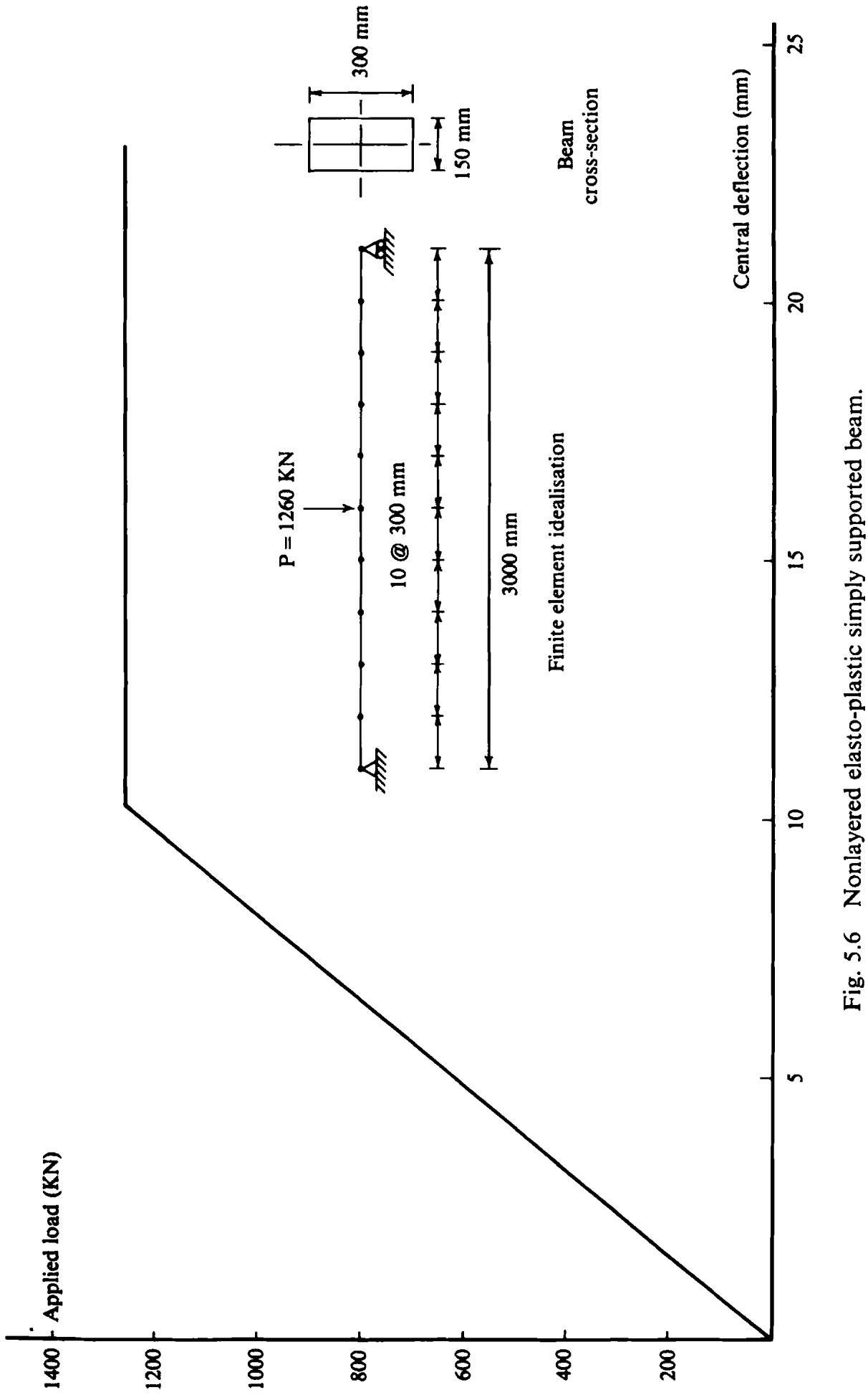
5.4.6 Examples of nonlayered elasto-plastic Timoshenko beam analysis Two numerical examples are considered. The first example, Example 5.1, involves the yielding of a rectangular simple beam under uniformly distributed load. The beam material has the following properties: $$ E = 2 1 0 \cdot 0 \mathrm{kN} / \mathrm{mm} ^ {2} $$ $$ \nu = 0 \cdot 3 $$ $$ \sigma_ {0} = 0 \cdot 2 5 \mathrm{kN} / \mathrm{mm} ^ {2} $$ $$ H ^ {\prime} = 0 \cdot 0 $$ and the beam proportions are: $$ b = 1 5 0 \mathrm{mm} $$ $$ t = 3 0 0 \mathrm{mm} $$ $$ l = 3 0 0 0 \mathrm{mm} $$ Typical input data is provided in Appendix IV. The problem, finite element idealisation employed and the results are illustrated in Fig. 5.6, which shows that the beam fails as soon as a plastic hinge forms at the centre of the beam. Note that the beam material is assumed to have no strain hardening. The second example considered, Example 5.2, is the clamped I beam shown in Fig. 5.7. The beam has the same material properties as those of Example 5.1. The dimensions and finite element discretisation of the beam are given in Fig. 5.7; the load-displacement relationship at the beam centre is also provided. It is seen that there is an initial loss of stiffness corresponding to the ![](images/page-149_e74f84438d5463fc913231dfde01b388b0d270c33f82df45ee677c8a957577fb.jpg)
line | Central deflection (mm) | Applied load (KN) | | ----------------------- | ----------------- | | 0 | 0 | | 10 | 1260 | | 10 @ 300 mm | 1260 | | 3000 mm | 1260 | | 300 mm | 1260 | | 150 mm | 1260 | | 300 mm | 1260 |
![](images/page-150_f09a675eb77b8f34b357f897f1326ccf573ece3513d714eca9a0076183984a4e.jpg) Fig. 5.7 Nonlayered elasto-plastic clamped beam.