```csv TTIME=TTIME+DTIME C C*** CALL ROUTINE WHICH SELECTS SOLUTION ALORITHM VARIABLE KRESL C CALL ALGOR(FIXED,IINCS,ISTEP,KRESL,TIMEX,MTOTV,NALGO,NTOTV) C*** CHECK WHETHER A NEW EVALUATION OF THE STIFFNESS MATRIX IS REQUIRED C IF(KRESL.EQ.1) CALL STIFVP(COORD,IINCS,LNODS,MATNO, MEVAB,MMATS,MPOIN,MTOTV,NELEM,NEVAB,NGAUS,NNODE, NSTRE,NSTR1,POSGP,PROPS,WEIGP,MELEM,MTOTG, STRSG,NTYPE,NCRIT,TIMEX,DTIME) C SOLVE EQUATIONS C CALL FRONT(ASDIS,ELOAD,EQRHS,EQUAT,ESTIF,FIXED,IFFIX,IINCS,ISTEP, GLOAD,GSTIF,LOCEL,LNODS,KRESL,MBUFA,MELEM,MEVAB,MFRON, MSTIF,MTOTV,MVFIX,NACVA,NAMEV,NDEST,NDOFN,NELEM,NEVAB, NNODE,NOFIX,NPIVO,NPOIN,NTOTV,TDISP,TLOAD,TREAC, VECRV) C C*** CALCULATE RESIDUAL FORCES C CALL STEPVP(ASDIS,COORD,ELOAD,ISTEP,LNODS,LPROP,TIMEX, MATNO,MELEM,MMATS,MPOIN,MTOTG,TAUFT,DTIME, MTOTV,NDOFN,NELEM,NEVAB,NGAUS,NNODE,NSTR1, NTYPE,POSGP,PROPS,NSTRE,NCRIT,STRSG,WEIGP, TDISP,VISTN,VIVEL,TLOAD,FTIME,DTINT,IINCS) C C*** CHECK FOR CONVERGENCE TO STEADY STATE C CALL STEADY(NELEM,NGAUS,NCHEK,VIVEL,ISTEP,FIRST,TOLER,PVALU, MTOTG,DTIME,NSTR1,TTIME) C C*** OUTPUT RESULTS IF REQUIRED C IF(NOUTP(1).EQ.0) GO TO 110 KOUTD=(ISTEP/NOUTP(1))*NOUTP(1) KOUTS=(ISTEP/NOUTP(2))*NOUTP(2) IF(KOUTD.NE.ISTEP.OR.KOUTS.NE.ISTEP) GO TO 110 KOUTP=2 IF(KOUTS.EQ.ISTEP) KOUTP=3 CALL OUTPUT(ISTEP,MTOTG,MTOTV,MVFIX,NELEM,NGAUS,NOFIX,NOUTP, NPOIN,NVFIX,STRSG,TDISP,TREAC,NTYPE,NCHEK,VIVEL, KOUTP) 110 CONTINUE C C*** IF SOLUTION HAS CONVERGED STOP ITERATING AND OUTPUT RESULTS C IF(NCHEK.EQ.0) GO TO 75 50 CONTINUE C C*** C 75 CALL OUTPUT(ISTEP,MTOTG,MTOTV,MVFIX,NELEM,NGAUS,NOFIX,NOUTP, NPOIN,NVFIX,STRSG,TDISP,TREAC,NTYPE,NCHEK,VIVEL, KOUTP) 100 CONTINUE STOP END VISC 65 VISC 66 VISC 67 VISC 68 VISC 69 VISC 70 VISC 71 VISC 72 VISC 73 VISC 74 VISC 75 VISC 76 VISC 77 VISC 78 VISC 79 VISC 80 VISC 81 VISC 82 VISC 83 VISC 84 VISC 85 VISC 86 VISC 87 VISC 88 VISC 89 VISC 90 VISC 91 VISC 92 VISC 93 VISC 94 VISC 95 VISC 96 VISC 97 VISC 98 VISC 99 VISC 100 VISC 101 VISC 102 VISC 103 VISC 104 VISC 105 VISC 106 VISC 107 VISC 108 VISC 109 VISC 110 VISC 111 VISC 112 VISC 113 VISC 114 VISC 115 VISC 116 VISC 117 VISC 118 VISC 119 VISC 120 VISC 121 VISC 122 VISC 123 VISC 124 ```

VISC 64	For each load increment, initialise the time step length.
VISC 65	Enter the time-stepping loop for the current load increment.
VISC 66	Compute the total time elapsed.
VISC 70	For the first timestep of the first load increment prepare for a full equation solution rather than a resolution for an explicit formulation. For the implicit or semi-implicit algorithm a complete equation solution is required each and every time-step.
VISC 73–85	Formulate the element stiffnesses and solve the resulting equations.
VISC 89–94	Calculate quantities at the end of the timestep and evaluate the loads for the next timestep.
VISC 98–99	Check for convergence of the time stepping process to steady state conditions.
VISC 103–105	Check to see if either displacement or stress output is required for this timestep.
VISC 106–107	Set KOUTP = 2 for displacement output only and KOUTP = 3 for both stress and displacement output.
VISC 108–110	Output the results.
VISC 115	If steady state conditions have been reached, output the converged results, increment the loads and proceed with the time-stepping process.

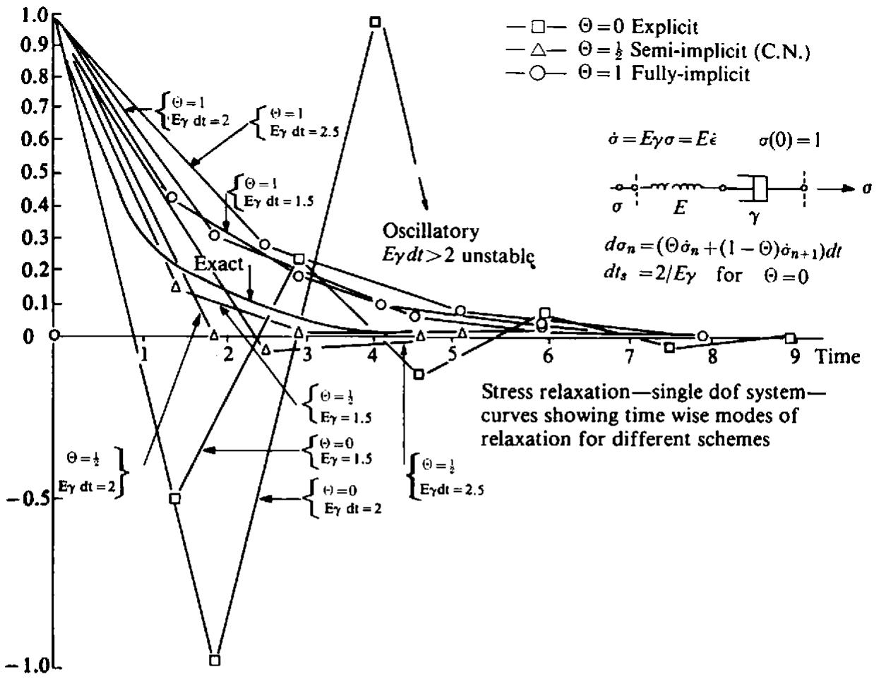
# 8.14 General comparison of implicit and explicit time integration schemes Before discussing the general case of a two-dimensional continuum it is instructive to consider the behaviour of a single degree of freedom system. In particular we will consider the response of a simple linear Maxwell model, as illustrated in Fig. 8.2. This situation is equivalent to the uniaxial viscoplastic model when the initial yield or threshold value, $F_{0}$ , is reduced to zero. Figure 8.2 shows the stress relaxation histories for different time integration schemes when the model is subjected to a constant total strain. It is observed that all results obtained using the fully implicit scheme ( $\Theta = 1$ ) lie to one side of the theoretical solution while the semi-implicit method ( $\Theta = \frac{1}{2}$ ) gives results which lie to either side of the true curve. It is also evident that the explicit method ( $\Theta = 0$ ) gives an oscillatory solution with the rate of convergence decreasing as the time step stability limit is approached. However, in each case the steady state solution is eventually correctly predicted. For the solution of elasto-plastic problems by use of the viscoplastic algorithm it is only the steady state solution that is of importance. Similarly in problems of creep, the transient stage may not be of interest in itself, as long as the steady state values are correctly arrived at. For problems which are geometrically linear the solution process simplifies considerably. The strain matrix $B^{n}$ is then constant throughout the analysis and from (8.19) it is seen to be equal to $B_{0}$ . For solution by the explicit time 

line

| Time | Θ = 0 Explicit | Θ = 1/2 Semi-implicit (C.N.) | Θ = 1 Fully-implicit | |------|----------------|------------------------------|------------------------| | 1 | 0.7 | 0.4 | 0.3 | | 2 | 0.5 | 0.2 | 0.1 | | 3 | 0.3 | 0.1 | 0.05 | | 4 | 0.1 | 0.05 | 0.02 | | 5 | 0.05 | 0.02 | 0.01 | | 6 | 0.02 | 0.01 | 0.005 | | 7 | 0.01 | 0.005 | 0.002 | | 8 | 0.005 | 0.002 | 0.001 | | 9 | 0.002 | 0.001 | 0.0005 |

Fig. 8.2 Characteristics of explicit and implicit time stepping algorithms when applied to a linear Maxwell model. marching scheme, $\Theta = 0$ and from (8.14) we have that $C^n = 0$ . Consequently, from (8.18), $\hat{D}^n = D$ and (8.24) implies that the tangential stiffness matrix becomes the linear elastic stiffness matrix and is constant throughout the solution process. Thus for the equation solution demanded by (8.23), a complete reduction and back-substitution is only required for the first time step and subsequent time intervals only require equation resolution. Experience to date $^{(2)}$ indicates that solution by the implicit method increases the computation time by approximately a factor of 4–5 in comparison with the explicit approach, for the same solution tolerance factor (or time step length). This cost differential must be balanced against the greater time step lengths permitted by the unconditionally stable implicit method. However, increasing the time step length beyond prescribed limits results in a deterioration in solution accuracy. Where a variable stiffness approach is employed for some other reasons, such as to include geometric nonlinearity effects or time dependent material properties, solution by an implicit scheme entails little or no additional computing effort and such an approach is particularly advantageous. Modification of the program presented to account for large deformation effects is set as an exercise to the reader in Section 8.17. Implicit and explicit time integration schemes are considered further in Chapters 10 and 11 for the solution of dynamic transient problems. # 8.15 The overlay method for improved material response The viscoplastic model described in the previous sections gives a material response whose general form is in keeping with experimental observations. However the precise strain/time histories (or creep curves) of many real materials cannot be accurately represented by a simple viscoplastic model. This is particularly so for materials whose strain response curves are nonlinear with regard to the applied stress level, so that a doubling of the applied stress does not result in twice the strain at any given time. A more elaborate material response can be modelled by use of the so-called overlay or mechanical sublayer method $^{(10-13)}$ in which the solid to be analysed is assumed to be composed of several layers or overlays each of which undergoes the same deformation. The total stress field is obtained by summing the different contributions of each overlay. By introducing a suitable number of overlays and assigning different material characteristics to each, a variety of sophisticated composite actions can be reproduced. In this section it is demonstrated how time-dependent overlay models can be used to simulate some experimentally observed material behaviours. 

flowchart

```mermaid graph TD A["Start"] -->|Primary creep| B["Stage B"] B -->|Secondary creep| C["Stage C"] C -->|Permanent set| D["Stage D"] D -->|Permanent set| E["Stage E"] E -->|Tertiary creep| F["Stage F"] F -->|Failure| G["Stage I"] style A fill:#f9f,stroke:#333 style B fill:#f9f,stroke:#333 style C fill:#f9f,stroke:#333 style D fill:#f9f,stroke:#333 style E fill:#f9f,stroke:#333 style F fill:#f9f,stroke:#333 style G fill:#f9f,stroke:#333 ```

Fig. 8.3 Strain/time relationship at constant stress for many typical materials. The strain-time relationship at constant stress which most materials exhibit to some degree or other is illustrated in Fig. 8.3. The instantaneous elastic strain, OA, is followed by a primary creep AB during which if unloading takes place an instantaneous elastic recovery results, followed by delayed elastic recovery, CD. If the load is not removed at time $T_{1}$ secondary creep begins which is accompanied by permanent deformation. Unloading at any time on the curve BE leaves a permanent set in the material. On continued loading past time $T_{2}$ tertiary creep begins, leading almost inevitably to failure. 

text_image

μ₁ μ₂ η

(a) Standard visco-elastic model 

text_image

μ₁ μ₂ η₂ Y η₁

(b) Four parameter model Fig. 8.4 Material models for simulation of the material behaviour of Fig. 8.3. (a) Standard visco-elastic model. (b) Four parameter model. This behaviour can be numerically simulated by use of the rheological models shown in Fig. 8.4. The standard linear solid illustrated in Fig. 8.4(a) provides a visco-elastic response and represents the behaviour of the material up to time $T_{1}$ . After this time the behaviour is closely approximated by the five parameter model shown in Fig. 8.4(b) where a friction slider component in parallel with a viscous dashpot has been added. This component becomes active only if the applied stress exceeds some limiting value, Y and the friction slider provides the permanent deformation or viscoplastic effect. For use in the overlay method it is desirable to consider ‘Maxwell equivalents’ of these models. Figure 8.5(a) shows the equivalent model to that of Fig. 8.4(a) both being governed by the differential equation $$ p _ {1} D \sigma + p _ {0} \sigma = q _ {1} D \epsilon + q _ {0} \epsilon , \tag {8.49} $$ where $p_{i}$ and $q_{i}$ are constants and D denotes the differential operator with respect to time. Similarly Fig. 8.5(b) illustrates the Maxwell equivalent of Fig. 8.4(b), the governing equation for this case being $$ p _ {2} D ^ {2} \sigma + p _ {1} D \sigma + p _ {0} \sigma = q _ {2} D ^ {2} \epsilon + q _ {1} D \epsilon + q _ {0} \epsilon . \tag {8.50} $$ 

text_image

μM η μH

(a) 

text_image

μM μH η Y* η' Hookean element

(b) Fig. 8.5 Equivalent representation of the models of Fig. 8.4 using Maxwell type components. The constants for the various components of the models in Figs. 8.4 and 8.5 are different but unique relationships exist. The configurations of Fig. 8.5 immediately suggest the use of overlay models. By employing at least one viscoplastic overlay and one Maxwell overlay (i.e. setting the threshold uniaxial yield value, $F_{0} = 0$ ) the complete behaviour in the visco-elastic range as well as irrecoverable creep deformation can be generated. The model behaves as a ‘standard linear solid’ until failure of the friction slider in the visco-plastic overlay after which it behaves as a four parameter solid. In fact a fifth parameter, the yield limit of the slider must also be defined. These parameters are material characteristics and their values must be experimentally determined. 

text_image

t_i l

Fig. 8.6 The overlay model in two-dimensional situations. # 8.15.1 Basic expressions of the overlay concept The overlay model in a two-dimensional situation is illustrated schematically in Fig. 8.6. Each overlay can have a different thickness and material behaviour. With the nodes in each overlay coincidental, the same strain pattern is produced in each component. This results in a different stress field $\sigma_{j}$ in each layer which contribute to the total stress field $\sigma$ according to the overlay thickness, $t_{j}$ , so that $$ \sigma = \sum_ {j = 1} ^ {k} \sigma_ {j} t _ {j}, \tag {8.51} $$ in which $k$ is the total number of overlays in the model, and $$ \sum_ {j = 1} ^ {k} t _ {j} = 1. \tag {8.52} $$ The equilibrium equations (8.21) which must be satisfied at each stage become $$ \int_ {\Omega} [ \boldsymbol {B} ^ {n} ] ^ {T} \sum_ {j = 1} ^ {k} \sigma_ {j} ^ {n} t _ {j} d \Omega + \boldsymbol {f} ^ {n} = \mathbf {0}. \tag {8.53} $$ Also the element stiffnesses (8.24) are the sum of each overlay contribution so that $$ \boldsymbol {K} _ {T} ^ {n} = \sum_ {j = 1} ^ {k} \int_ {\Omega} [ \boldsymbol {B} ^ {n} ] ^ {T} (\boldsymbol {D} ^ {n}) _ {j} \boldsymbol {B} ^ {n} d \Omega , \tag {8.54} $$ where $(\hat{D}^{n})_{j}$ is the value of $\hat{D}^{n}$ for each overlay in turn. Matrix $(\hat{D}^{n})_{j}$ will differ from overlay to overlay according to the material properties of each. The solution process is then identical to that described in the preceding sections with stress and strain terms being calculated for each overlay separately. It should be noted that the viscoplastic strain in each overlay will generally be different due to differences in threshold yield values and flow rates but the total strains must be the same. Although the name overlay model arises from the physical interpretation of the two-dimensional situation the technique is essentially a mathematical convenience and can be readily extended to three-dimensional problems. In such cases the thickness can no longer be interpreted as a physical quantity and becomes merely a weighting parameter for combining the contribution of individual overlays. Indeed this is also the case in two-dimensional problems where negative thicknesses can be employed to simulate strain-softening conditions. $^{(12)}$ # 8.15.2 Overlay models for some standard material behaviours In this section we reproduce some standard material responses by combining different viscoplastic components through the overlay concept. $^{(13)}$  Fig. 8.7 Use of the overlay concept for the simulation of some standard material behaviours. # (i) Visco-elastic response A two overlay model with $F_{0}$ set to zero for one overlay and infinitely large in the other reproduces a standard linear visco-elastic solid (Fig. 8.7). Any higher order time dependent constitutive relation can be simulated by the introduction of more overlays of the Maxwell type (i.e. $F_{0} = 0$ ). Quite generally a stress–strain relationship of the form $$ \sum_ {k = 0} ^ {n} a _ {k} D ^ {k} \sigma = \sum_ {k = 0} ^ {n} a _ {k} D ^ {k} \epsilon , \tag {8.55} $$ in which $a_{k}$ and $b_{k}$ are real valued functions of the spatial coordinates and D denotes the differential time operator, can be modelled by the use of n Maxwell type overlays. The overlay approach reduces the $n^{th}$ order differential equation (8.55) to n first order equations. # (ii) Four parameter viscous model Two overlays with $F_{0}$ set to zero in each case provides a four parameter viscous model of the first kind (Fig. 8.7). Three overlays with $F_{0}$ set to (a) zero for one overlay (b) infinitely large for the second unit, (c) zero for the third overlay together with a small prescribed elastic modulus, reproduces a four parameter model of the second kind. # (iii) Three element viscous model A two overlay model with $F_{0}$ set to zero in both and the elastic modulus assigned to be infinitely large in one reproduces the three element viscous model. # (iv) Visco-elastic-plastic four parameter model This two overlay model is capable of reproducing the behaviour of most real engineering materials and is achieved by setting the threshold yield value of one overlay to zero. Before yielding of the friction slider, the material behaviour is visco-elastic followed by a viscoplastic response after initial yielding. By choosing the viscosity coefficients of the two dashpots appropriately the rate of straining after first yield can be controlled. In order to illustrate how the combination of two simple material responses by the overlay method can simulate a more complex material behaviour the load cycling problem indicated in Fig. 8.8 is presented. One elastic (yield value set very large) and one viscoplastic overlay are considered. A static analysis of the load cycling of this model was performed by allowing steady state conditions to be achieved after application of each increment of load. The results are shown in Fig. 8.8 where the material properties employed are also included. A Bauschinger effect is immediately apparent on reversal of loading with yielding in compression commencing at a reduced value compared with initial yield in tension. Thus although each overlay has been assumed to be non-strain hardening with equal yield stress in tension and compression, the composite model exhibits a kinematic hardening behaviour. As a further demonstration of the overlay approach, Fig. 8.9 shows how two overlays can be used to simulate the response of a real engineering material. The solid lines represent experimentally obtained creep curves for a rock salt and it is evident that the material behaviour is highly nonlinear with regard to the strain obtained at any time for a given applied load. The broken lines are the numerical material response obtained by using two overlays with material properties as shown in Fig. 8.9. The agreement obtained is acceptable for engineering purposes but a closer correspondence could be readily achieved by the use of additional overlays. The main advantage of the overlay technique is that it allows the description of complex material behaviours by the use of components which individually exhibit a simple response. All the program changes required to implement the overlay method in the viscoplastic program described earlier in this chapter are of a minor nature. Almost all the changes are associated with the summation process over each overlay demanded by (8.51), (8.53) and (8.54). Several array sizes must also be extended to allow separate storage of quantities for each overlay. Modification of the program is set as an exercise for the reader in Section 8.17. # 8.16 Numerical examples The first problem considered is the elasto-viscoplastic deformation of a thick tube under the action of internal pressure loading with the exterior surface remaining free. The mesh of Fig. 7.12(a) is employed in analysis with 

line

| ε/ε₀ | σ/Yₐ | |------|------| | -1.5 | -1.5 | | -1.0 | -1.0 | | -0.5 | -0.5 | | 0.0 | 0.0 | | 0.5 | 0.5 | | 1.0 | 1.0 | | 1.5 | 1.5 | | 2.0 | 2.0 |

Fig. 8.8 Load cycling response of an overlay composite illustrating the Bauschinger effect.