# Chapter 11 Implicit-explicit transient dynamic analysis Written in collaboration with D. K. Paul # 11.1 Introduction In Chapter 10 we have shown that the explicit, central difference time stepping scheme is a simple and powerful method of time integration. The main drawback of the scheme is that it is conditionally stable. Thus the computational advantages of the central difference scheme are counterbalanced by the very small size of time step necessary when some stiff (and/or small) elements are present. For such problems the unconditionally stable implicit schemes permit the use of larger time steps, the size of which is governed only by accuracy considerations. Unfortunately these schemes which require matrix factorisations involve larger computer core storage and more operations per time step than the central difference scheme. The selection of a suitable time integration scheme is therefore largely a matter of experience. In some problems, typified by the one illustrated in Fig. 11.1, we may be confronted with a situation in which there is a 'soft' subregion $\Omega^{E}$ where an ![](images/page-441_8f75f37bc4258965dd48ad992b15d6e07ae58b7e496007f37154a7493422bbbb.jpg)
text_image Implicit subregion, Ω′ Explicit subregion, Ω^ε
Fig. 11.1 Implicit-explicit partitioning. explicit scheme is desirable and a 'stiff' subregion $\Omega^I$ where an implicit scheme is preferable for greater efficiency. In such cases it is possible to simultaneously make use of both implicit and explicit algorithms. Implicit-explicit schemes offer a unified approach to problems of structural transient dynamics and can lead to significant computational advantages. Implicit-explicit schemes were first introduced by Belytschko and Mullen $^{(1-3)}$ and were given an alternative form by Hughes and co-workers $^{(4-6)}$ and Park et al. $^{(7-8)}$ It can be shown that the stability of such schemes is governed by the explicit elements. In this chapter Implicit and Implicit-Explicit methods for nonlinear transient dynamic analysis are discussed and we follow the element partitioning approach described by Hughes. A program, named MIXDYN, for Implicit-Explicit linear and nonlinear transient dynamic analysis is included. Some numerical examples are solved to show some of the capabilities of the program. The same program could be modified for static analysis by some simple changes. # 11.2 Implicit time integration # 11.2.1 Newmark's algorithm In order to introduce the implicit/explicit algorithm we describe the predictor-corrector form of the Newmark scheme for the integration of the semi-discrete system of equations which govern nonlinear transient dynamic problems. Typically at time station $t_{n} + \Delta t$ these equations take the form $$ \boldsymbol {M} \boldsymbol {a} _ {n + 1} + \boldsymbol {p} _ {n + 1} = \boldsymbol {f} _ {n + 1} \tag {11.1} $$ where $M, a_{n+1}, p_{n+1}$ and $f_{n+1}$ are the mass matrix, acceleration vector, internal force vector (which may depend on the displacements $d_{n+1}$ and velocities $\dot{d}_{n+1}$ and their histories) and applied force vector respectively. Let $$ [ \boldsymbol {K} _ {T} ] _ {n + 1} = \partial \boldsymbol {p} _ {n + 1} / \partial \boldsymbol {d} _ {n + 1} \text { and } [ \boldsymbol {C} _ {T} ] _ {n + 1} = \partial \boldsymbol {p} _ {n + 1} / \partial \dot {\boldsymbol {d}} _ {n + 1} \tag {11.2} $$ denote the tangent stiffness and damping matrices respectively. In the Newmark scheme we endeavour to satisfy the following equations $$ \boldsymbol {M} \boldsymbol {a} _ {n + 1} + \boldsymbol {p} _ {n + 1} = \boldsymbol {f} _ {n + 1} \tag {11.3} $$ $$ \boldsymbol {d} _ {n + 1} = \tilde {\boldsymbol {d}} _ {n + 1} + \Delta t ^ {2} \beta \boldsymbol {a} _ {n + 1} \tag {11.4} $$ $$ \boldsymbol {v} _ {n + 1} = \widetilde {\boldsymbol {v}} _ {n + 1} + \Delta t \gamma \boldsymbol {a} _ {n + 1} \tag {11.5} $$ where $$ \tilde {\boldsymbol {d}} _ {n + 1} = \boldsymbol {d} _ {n} + \Delta t \boldsymbol {v} _ {n} + \Delta t ^ {2} (1 - 2 \beta) \boldsymbol {a} _ {n} / 2 \tag {11.6} $$ $$ \widetilde {v} _ {n + 1} = v _ {n} + \Delta t (1 - \gamma) a _ {n}. \tag {11.7} $$ Note that $d_{n}$ , $v_{n}$ and $a_{n}$ are the approximations to $d(t_{n})$ , $\dot{d}(t_{n})$ and $\ddot{d}(t_{n})$ and $\beta$ and $\gamma$ are free parameters which control the accuracy and stability of the method. The values $\tilde{d}_{n+1}$ and $\tilde{v}_{n+1}$ are predictor values and $d_{n+1}$ and $v_{n+1}$ are corrector values. Initially the displacements $d_{0}$ and velocities $v_{0}$ are provided and we find the accelerations $a_{0}$ from the expression $$ \boldsymbol {M} \boldsymbol {a} _ {0} = \boldsymbol {f} _ {0} - \boldsymbol {p} (\boldsymbol {d} _ {0}, \boldsymbol {v} _ {0}). \tag {11.8} $$ Thus $a_{0}$ may be found by a factorization, forward reduction and back substitution unless M is diagonal in which case the solution is trivial. We then solve (11.3) to (11.7) by forming an ‘effective static problem’† which is solved using a Newton Raphson type scheme, as described earlier. The algorithm is summarised in Table 11.1. Table 11.1 Newmark's algorithm
1Set iteration counter i = 0.
2Begin predictor phase in which we set
$d_{n+1}^{[i]} = \tilde{d}_{n+1} = d_n + \Delta tv_n + \Delta t^2(1-2\beta)a_n/2$ (i)
$v_{n+1}^{[i]} = \tilde{v}_{n+1} = v_n + \Delta t(1-\gamma)a_n$ (ii)
$a_{n+1}^{[i]} = [d_{n+1}^{[i]} - \tilde{d}_{n+1}]/(\Delta t^2\beta) = 0.$ (iii)
3Evaluate residual forces using the equation
$\psi^{[i]} = f_{n+1} - Ma_{n+1}^{[i]} - p(d_{n+1}^{[i]}, v_{n+1}^{[i]}).$ (iv)
4If required, form the effective stiffness matrix using the expression
$K^* = M/(\Delta t^2\beta) + \gamma C_T/(\Delta t\beta) + K_T(d_{n+1}^{[i]}).$ (v)
Otherwise use a previously calculated $K^*$ .
5Factorize, forward reduction and backsubstitute as required to solve
$K^* \Delta d^{[i]} = \psi^{[i]}$ .(vi)
6Enter corrector phase in which we set
$d_{n+1}^{[i+1]} = d_{n+1}^{[i]} + \Delta d^{[i]}$ (vii)
$a_{n+1}^{[i+1]} = [d_{n+1}^{[i+1]} - \tilde{d}_{n+1}]/(\Delta t^2\beta)$ (viii)
$v_{n+1}^{[i+1]} = v_{n+1} + \Delta t\gamma a_{n+1}^{[i+1]}$ .(ix)
7If $\Delta d^{[i]}$ and/or $\psi^{[i]}$ do not satisfy the convergence conditions then set i = i+1 and go to step 3, otherwise continue.
8Set(x)
$d_{n+1} = d_{n+1}^{[i+1]}$ (xi)
$v_{n+1} = v_{n+1}^{[i+1]}$ (xii)
$a_{n+1} = a_{n+1}^{[i+1]}$
for use in the next time step. Also set n = n+1, form p and begin next time step.
\* In this chapter $\gamma$ is a Newmark parameter and not the viscoplastic fluidity parameter. $\dagger K^{*}\Delta d^{[i]} = \psi^{[i]}$ . # 11.2.2 Predictor-corrector algorithm Let us now consider an 'explicit' algorithm associated with the Newmark schemes described earlier. In this explicit predictor-corrector algorithm we assume that the mass matrix $M$ is diagonal and we make use of the expression $$ M a _ {n + 1} + p \left(\tilde {d} _ {n + 1}, \tilde {v} _ {n + 1}\right) = f _ {n + 1} \tag {11.9} $$ Notice that the calculation is explicit since we use corrector values obtained from information given in the previous step. As we would like to eventually combine the implicit and explicit methods we organise our implementation of this explicit method in a similar fashion to the implementation given of the implicit scheme in the previous section. Table 11.2 summarises the algorithm. Table 11.2 Explicit predictor-corrector algorithm
1Begin predictor phase by setting $d_{n+1}^{[0]} = \tilde{d}_{n+1} = d_n + \Delta t v_n + \Delta t^2 (1 - 2\beta) a_n / 2$ (i) $v_{n+1}^{[0]} = \tilde{v}_{n+1} = v_n + \Delta t (1 - \gamma) a_n$ (ii) $a_{n+1}^{[0]} = 0.$ (iii)
2Evaluate the residual forces using the equation $\psi^{[0]} = f_{n+1} - p(d_{n+1}^{[0]}, v_{n+1}^{[0]}).$ (iv)
3If required, form the ‘effective’ stiffness matrix using the expression $K^* = M / (\Delta t^2 \beta).$ (v)Note that as the mass matrix $M$ does not change $K^*$ will be formed once only.
4Perform factorization, forward reduction and backsubstitution as required to solve $K^* \Delta d^{[0]} = \psi^{[0]}$ (vi)
5Enter the corrector phase in which we set $d_{n+1}^{[1]} = d_{n+1}^{[0]} + \Delta d^{[0]}$ (vii) $a_{n+1}^{[1]} = [d_{n+1}^{[1]} - \tilde{d}_{n+1}] / (\Delta t^2 \beta)$ (viii) $v_{n+1}^{[1]} = v_{n+1} + \Delta t \gamma a_{n+1}^{[1]}$ . (ix)
6Set $d_{n+1} = d_{n+1}^{[1]}$ (x) $v_{n+1} = v_{n+1}^{[1]}$ (xi) $a_{n+1} = a_{n+1}^{[1]}$ (xii)for use in the next time step. Also set $n = n+1$ , form $p$ and begin next time step.
# 11.3 Implicit-explicit algorithm # 11.3.1 Introduction We now combine the methods described in Sections 11.2.1 and 11.2.2 so that the finite element mesh contains two groups of elements: the implicit group and the explicit group. The superscripts I and E will henceforth refer to the implicit and explicit groups respectively. In the implicit-explicit algorithm we iterate within each time step in order to satisfy the equation $$ M a _ {n + 1} + p ^ {I} (d _ {n + 1}, v _ {n + 1}) + p ^ {E} (\tilde {d} _ {n + 1}, \tilde {v} _ {n + 1}) = f _ {n + 1} \tag {11.10} $$ in which $M = M^{I} + M^{E}$ and $f_{n+1} = f_{n+1}^{I} + f_{n+1}^{E}$ . Note that we assume $M^{E}$ is diagonal. # 11.3.2 The structure of the effective stiffness matrix The algorithm, which is summarised in Table 11.3, is very similar to the implicit algorithm given in Section 11.2.2. The profile structure of $K^{*}$ is very interesting. It has diagonal subregions corresponding to the explicit group of elements. Elsewhere, $K^{*}$ has a profile structure which corresponds to the connectivity of the implicit group only. Table 11.3 Implicit-explicit algorithm
1Set iteration counter i = 0.
2Begin predictor phase in which we set
$d_{n+1}^{[i]} = \tilde{d}_{n+1} = d_n + \Delta tv_n + \Delta t^2(1-2\beta)a_n/2$ (i)
$v_{n+1}^{[i]} = \tilde{v}_{n+1} = v_n + \Delta t(1-\gamma)a_n$ (ii)
$a_{n+1}^{[i]} = [d_{n+1}^{[i]}-d_{n+1}]/(\Delta t^2\beta) = 0.$ (iii)
3Evaluate residual forces using the equation
$\psi^{[i]} = f_{n+1} - Ma_{n+1}^{[i]} - p^I(d_{n+1}^{[i]}, v_{n+1}^{[i]}) - p^E(\tilde{d}_{n+1}, \tilde{v}_{n+1}).$ (iv)
4If required, form the effective stiffness matrix using the expression
$K^* = M/(\Delta t^2\beta) + \gamma C_T^I/(\Delta t\beta) + K_T^I(d_{n+1}^{[i]}).$ (v)
Otherwise use a previously calculated $K^*$ .
(Note that $K_T^I = \partial p^I/\partial d$ and $C_T^I = \partial p^I/\partial v$ ).
5Perform factorization, forward reduction and backsubstitution as required to solve
$K^* \Delta d^{[i]} = \psi^{[i]}$ .(vi)
6Enter corrector phase in which we set
$d_{n+1}^{[i+1]} = d_{n+1}^{[i]} + \Delta d^{[i]}$ (vii)
$a_{n+1}^{[i+1]} = [d_{n+1}^{[i+1]} - \tilde{d}_{n+1}]/(\Delta t^2\beta)$ (viii)
$v_{n+1}^{[i+1]} = v_{n+1} + \Delta t\gamma a_{n+1}^{[i+1]}$ .(ix)
7If $\Delta d^{[i]}$ and/or $\psi^{[i]}$ do not satisfy the convergence conditions, then set i = i+1 and go to step 3, otherwise continue.
8Set(x)
$d_{n+1} = d_{n+1}^{[i+1]}$ (xi)
$v_{n+1} = v_{n+1}^{[i+1]}$ (xii)
$a_{n+1} = a_{n+1}^{[i+1]}$
for use in the next time step. Also set n = n+1, form p and begin next time step.
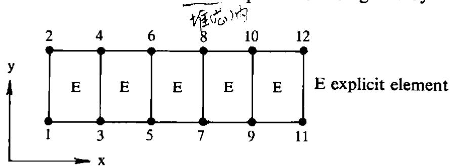
Consider the three meshes and effective stiffness matrices shown in Fig. 11.2(a)–(c): (i) When there are only explicit elements, $K^*$ is diagonal. In other words $K^*$ has the same profile structure as $M^E$ (Fig. 11.2(a)). (ii) For a mesh consisting of only implicit elements $K^*$ has the same profile structure as $K^I$ (Fig. 11.2(b)). (iii) For the partitioned mesh containing both implicit and explicit groups we see the appropriate combination of parts of both profile structures (Fig. 11.2(c)). To fully exploit the profile structure of $K^*$ , Hughes et al. (4) have suggested the use of profile solvers. In our implementation of the scheme we adopt a slightly modified version of the in-core profile solver given by Bathe and Wilson. (9) ![](images/page-446_73ac69057b6675d7707844c33ea3e53f989601f28d8d633f4ff7433df51a5ee7.jpg)
text_image 堆芯内 2 4 6 8 10 12 E E E E E E explicit element 1 3 5 7 9 11 x
(i) Finite element mesh—2 degrees of freedom per node. ![](images/page-446_0e03a8892b0b392a9b767e2f1e80c60951e1345af7210eb052fb2ad71e405493.jpg)
line | Equation number | Value | | --------------- | ----- | | 1 | × | | 2 | × | | 3 | × | | 4 | × | | 5 | × | | 6 | × | | 7 | × | | 8 | × | | 9 | × | | 10 | × | | 11 | × | | 12 | × | | 13 | × | | 14 | × | | 15 | × | | 16 | × | | 17 | × | | 18 | × | | 19 | × | | 20' | × | | 21 | × | | 22 | × | | 23 | × | | 24 | × |
Fig. 11.2(a) Two-dimensional finite element mesh and profile structure of the effective stiffness matrix $K^{*}$ (explicit elements only). # 11.3.3 Alternative predictor values In equations (i)–(iii) in Table 11.3 we gave the approach described by Hughes and Liu. $^{(4)}$ For implicit–explicit problems other predictor values may be adopted. Here we consider two cases: 1. Hughes and Liu predictor values $$ \boldsymbol {d} _ {n + 1} ^ {[ 0 ]} = \tilde {\boldsymbol {d}} _ {n + 1} = \boldsymbol {d} _ {n} + \Delta t \boldsymbol {v} _ {n} + \Delta t ^ {2} (1 - 2 \beta) \boldsymbol {a} _ {n} / 2 \tag {i} $$ $$ \boldsymbol {v} _ {n + 1} ^ {[ 0 ]} = \widetilde {\boldsymbol {v}} _ {n + 1} = \boldsymbol {v} _ {n} + \Delta t (1 - \gamma) \boldsymbol {a} _ {n} \tag {ii} $$ $$ \boldsymbol {a} _ {n + 1} ^ {[ 0 ]} = \left[ \boldsymbol {d} _ {n + 1} ^ {[ 0 ]} - \tilde {\boldsymbol {d}} _ {n + 1} \right] / \left(\Delta t ^ {2} \beta\right) \tag {iii} $$ ![](images/page-448_b37c753784b44147b038362413d309dfe84c50fb22f6d73cad1bdb9ba7eb6d9b.jpg)
text_image 2 4 6 8 10 12 y E E I I E 1 3 5 7 9 11 x E explicit element I implicit element
(i) Finite element mesh—2 degrees of freedom per node. ![](images/page-448_b789f654a0a1753921fc63f9661e18d78f2c5d0244652165acdeaad4670a92d0.jpg) (ii) Profile of $K^{*}$ . Fig. 11.2(c) Two-dimensional finite element mesh and profile structure of the effective stiffness matrix $K^{*}$ (Implicit and explicit elements). If $\gamma\geqslant\frac{1}{2}$ and $\beta=(\gamma+\frac{1}{2})^{2}/4$ , we achieve unconditional stability in the implicit element group. The time step is then restricted by the explicit element group. For the case in which $\gamma=\frac{1}{2}$ , the critical time step may be written as $$ \Delta t _ {\mathrm{crit}} = 2 / \omega_ {\max} \tag {11.13} $$ where $\omega_{max}$ is the maximum frequency of the explicit group. We can estimate $\omega_{max}$ as $$ \omega_ {\max} \leqslant \max _ {e} \left(\omega_ {\max} ^ {(e)}\right) \tag {11.14} $$ where $\omega_{\max}^{(e)}$ is the maximum frequency of the $e^{th}$ element of the explicit group. Since $K_{T}$ is changing from step to step, strictly speaking the maximum frequency should be estimated at the beginning of every step. In elastoplastic analysis, the structure generally becomes more flexible and (11.14) may be used. However, for a better estimate of the critical time step the nonlinear eigenvalues should be evaluated. If only implicit elements are used and if $\gamma\geqslant\frac{1}{2}$ and $\beta=(\gamma+\frac{1}{2})^{2}/4$ , then error investigations carried out in terms of period elongation and amplitude decay with the increase of time step indicate that for reasonable accuracy the time step should be limited to 1/100 of the fundamental (largest) period. It is observed that the amplitude decay caused by the numerical integration errors effectively filters the higher mode response out of the solution in the Houbolt and Wilson $\theta$ method. However when we employ the Newmark constant–average–acceleration scheme, which does not introduce amplitude decay, the higher frequency response is retained in the solution. In order to obtain amplitude decay using the Newmark method, it is necessary to employ $\gamma>\frac{1}{2}$ . # 11.4 Evaluation of the tangential stiffness matrix In program MIXDYN we adopt an elasto-plastic material model and therefore the stresses and the tangential stiffness matrix at any time station $t_{n}+\Delta t$ may be evaluated in the manner outlined in Chapter 7 for static problems. As an alternative geometrically nonlinear elastic effects are considered using a total Lagrangian formulation. The internal resisting force vector for the implicit elements at time station $t_{n} + \Delta t$ is given as $$ \boldsymbol {p} _ {n + 1} ^ {I} = \int_ {\Omega^ {I}} [ \boldsymbol {B} ^ {I} ] ^ {T} _ {n + 1} \sigma_ {n + 1} d \Omega \tag {11.15} $$ and therefore the tangential stiffness matrix may be written as $$ \begin{array}{l} \frac {\partial \boldsymbol {p} _ {n + 1} ^ {I}}{\partial \boldsymbol {d} _ {n + 1}} = [ \boldsymbol {K} _ {T} ^ {I} ] _ {n + 1} = \int_ {\Omega^ {I}} [ \boldsymbol {B} ^ {I} ] ^ {T} _ {n + 1} \boldsymbol {D} _ {n + 1} [ \boldsymbol {B} ^ {I} ] _ {n + 1} d \Omega \\ + \int_ {\Omega^ {I}} [ \boldsymbol {G} ] ^ {T} _ {n + 1} \boldsymbol {S} _ {n + 1} \boldsymbol {G} _ {n + 1} d \Omega \tag {11.16} \\ \end{array} $$ in which $D_{n+1}$ is the elasto-plastic modulus matrix defined in Chapter 7, $[B_{NL}^I]_{n+1}$ is the nonlinear strain-displacement matrix defined in Chapter 10, the matrix $S_{n+1}$ is given as $$ \boldsymbol {S} _ {n + 1} = \left[ \begin{array}{l l} \sigma_ {x} \boldsymbol {I} _ {2} & \tau_ {x y} \boldsymbol {I} _ {2} \\ \tau_ {x y} \boldsymbol {I} _ {2} & \sigma_ {y} \boldsymbol {I} _ {2} \end{array} \right] _ {n + 1} \tag {11.17} $$ for plane stress and plane strain problems, and $$ \boldsymbol {S} _ {n + 1} = \left[ \begin{array}{c c c} \sigma_ {r} \boldsymbol {I} _ {2} & \tau_ {r z} \boldsymbol {I} _ {2} & \boldsymbol {0} \\ \tau_ {r z} \boldsymbol {I} _ {2} & \sigma_ {z} \boldsymbol {I} _ {2} & \boldsymbol {0} \\ \boldsymbol {0} & \boldsymbol {0} & \sigma_ {\theta} \end{array} \right] _ {n + 1} \tag {11.18} $$ \* The second matrix is only included for geometrically nonlinear problems. for axisymmetric problems, and $$ [ G _ {i} ] _ {n + 1} = \left[ \begin{array}{c c c c} \frac {\partial N _ {i}}{\partial x} & 0 & \frac {\partial N _ {i}}{\partial y} & 0 \\ 0 & \frac {\partial N _ {i}}{\partial x} & 0 & \frac {\partial N _ {i}}{\partial y} \end{array} \right] ^ {T} \tag {11.19} $$ for plane stress and plane strain problems, and $$ [ G _ {i} ] _ {n + 1} = \left[ \begin{array}{c c c c c} \frac {\partial N _ {i}}{\partial r} & 0 & \frac {\partial N _ {i}}{\partial z} & 0 & \frac {N _ {i}}{r} \\ 0 & \frac {\partial N _ {i}}{\partial r} & 0 & \frac {\partial N _ {i}}{\partial z} & 0 \end{array} \right] ^ {T} \tag {11.20} $$ for axisymmetric problems. Note that all of the yield criteria described in Chapter 7 are included in program MIXDYN. # 11.5 Program MIXDYN # 11.5.1 Introduction The computer program 'MIXDYN' is based on the Implicit-Explicit time integration scheme of Hughes and Liu $^{(4)}$ for two-dimensional plane stress/strain and axisymmetric nonlinear dynamic transient problems. Some of the subroutines are the same as in DYNPAK. The profile solvers DECOMP and REDBAK and a few other subroutines used in this program are based on those given in Reference (9). (These subroutines are rewritten using new variables names). Some new subroutines have also been included in the program. The program considers geometric or elasto-plastic material nonlinearity. A total Lagrangian formulation using four-, eight- and nine-noded quadrilateral isoparametric elements is adopted to model the geometric nonlinear behaviour. The program has several options; it can be used for small or large deformation elastic and small deformation elasto-plastic transient dynamic analysis and the analysis may be carried out using an explicit, implicit or combined implicit-explicit algorithm. Furthermore, four types of elasto-plastic material models can be considered: (i) Tresca, (ii) Von Mises, (iii) Drucker-Prager and (iv) Mohr-Coulomb. The flow diagram for MIXDYN is shown in Fig. 11.3. The program is written in modular form and the input and output data representation is identical to that given for DYNPAK. The subroutines which have not appeared elsewhere in the book are now described.